Variational Autoencoders Explained

1. Overview

1.1. What are VAEs?

A Variational Autoencoder (VAE) is a generative model that learns a compressed, continuous representation (a latent space) of data. It consists of an encoder network that maps data to a distribution in the latent space and a decoder network that reconstructs data from samples drawn from that latent distribution.

1.2. Original Motivation

VAEs were designed to overcome a key limitation of standard autoencoders: the lack of a structured latent space that could be easily sampled from to generate new data. By introducing a probabilistic approach, VAEs ensure the latent space is continuous and organized, allowing for meaningful interpolation and the generation of novel, realistic data points. This probabilistic framework also provides a principled way to learn a compressed representation of the data.

1.3. Relevant Papers

Kingma, D.P., & Welling, M. (2013) – “Auto-Encoding Variational Bayes”: This is the original paper that introduced the VAE, framing the problem of learning a deep generative model as an optimization of a lower bound on the data log-likelihood (the Evidence Lower Bound, or ELBO).
Rezende, D.J., Mohamed, S., & Wierstra, D. (2014) – “Stochastic Backpropagation and Variational Inference”: Published independently, this paper proposed a similar framework, also using the reparameterization trick to make backpropagation through the sampling process possible.

1.4. Current Status

VAEs remain a cornerstone of deep generative modeling. They’re a foundational model taught in machine learning courses and are continuously being improved upon. Research focuses on addressing limitations like generating blurry outputs and improving the fidelity of the latent space representation. Extensions include conditional VAEs (CVAEs) and discrete VAEs. VAEs are often used as a baseline or a component in more complex generative models like normalizing flows.

1.5. Relevance

VAEs are highly relevant for their ability to learn an interpretable latent space. Unlike GANs, which can be unstable to train and often have a chaotic latent space, VAEs provide a smooth and continuous manifold. This makes them ideal for tasks like data visualization, anomaly detection, and controlled data generation (e.g., generating a “happy” face with “glasses” by moving along specific latent dimensions). They also have a clear theoretical foundation based on variational inference, which provides a measure of how well the model fits the data.

1.5. Applications

1.4. Current Status

1.5. Relevance

1.5. Applications

Image Generation & Manipulation: Used for generating new images, and for tasks like “style transfer” and “face editing” by manipulating the latent representation. Anomaly Detection: By measuring the reconstruction error or the distance of a data point from the learned distribution in the latent space, VAEs can effectively identify outliers. Drug Discovery & Molecular Design: VAEs can learn a latent representation of molecules, allowing researchers to explore the space of possible molecules and design new ones with desired properties. Audio Synthesis: Used to generate new sounds, music, and speech by learning a latent space representation of audio signals.

2. From GMMs to VAEs: Discrete vs. Continuous Latent Space

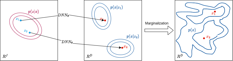
In the last post, we dealt with the GMMs log-likelihood. We fit the model by solving the optimization problem using the EM algorithm. In the E-step, we mentioned that we need to evaluate the posterior to formulate the Q-function. In the case of GMMs, we were able to evaluate it because GMMs assume that the latent space is discrete, meaning the latent variable is discrete and can only take on a finite number of distinct values (the cluster index for GMMs): \[ P(z=k|x) = \frac{P(x|z=k) \cdot P(z=k)}{P(x)} = \frac{P(x|z=k) \cdot P(z=k)}{\sum_{k=1}^{K} P(x|z=k) \cdot P(z=k)} \] Usually, if we sample from a continuous latent space, we can improve the quality of the representation. However, this comes at the cost of an intractable log-likelihood with no closed-form solution. When the latent variable \( z \) is continuous, the marginalization expression becomes an integral over this continuous space. This will make the evaluation of the posterior intractable, and we won’t be able to solve the optimization problem with the EM algorithm, for example: \[ P(z|x) = \frac{P(x|z) \cdot P(z)}{P(x)} = \frac{P(x|z) \cdot P(z)}{\int P(x|z) \cdot P(z) \,dz} \] In this case, we need approximation methods to handle the intractable integral in the posterior calculation.

3. Variational Inference

Variational inference is an approach to approximate the posterior distribution \( p(z|x) \) when computing it explicitly is intractable. We define an approximate posterior \( q(z|x) \) and we find it by solving an optimization problem that seeks to minimize the disparity between the true and approximate posterior. A measure of disparity is the Kullback-Leibler divergence.

3.1. KL Divergence

Kullback-Leibler divergence \( D_{KL} \) is a statistical measure of how two probability distributions are different from each other. It is also related to information theory, as it is also known as relative entropy, which quantifies the information lost when using a distribution \( Q \) to approximate a true distribution \( P \). In the variational inference context, we minimize \( D_{KL}(q(z|x) || p(z|x)) \) to find the best approximate or variational posterior \( q(z|x) \): \[ \begin{align*} D_{KL}(q(z|x) || p(z|x)) &= E_{z \sim q}\left[ \log \frac{q(z|x)}{p(z|x)} \right] \\ &= E_{z \sim q}\left[ \log q(z|x) – \log \frac{p(x,z;\theta)}{p(x;\theta)} \right] \\ &= E_{z \sim q}\left[ \log q(z|x) \right] – E_{z \sim q}\left[ \log p(x,z;\theta) \right] + E_{z \sim q}\left[ \log p(x;\theta) \right] \\ &= \log p(x;\theta) – E_{z \sim q}\left[ \log \frac{p(x,z;\theta)}{q(z|x)} \right] \\ &= \log \text{likelihood} – \text{ELBO} \end{align*} \]

3.2. ELBO: Evidence Lower Bound

From the above derivation, we conclude that: \( \log \text{likelihood} = D_{KL} + \text{ELBO} \). ELBO is called the Evidence Lower Bound. It is called so because in the context of Bayesian inference, the (log)-likelihood corresponds to the evidence. Additionally, \( D_{KL} \) is always positive, which means ELBO is a lower bound on the log-likelihood, where \( D_{KL} \) is the gap between them. Instead of evaluating the log-likelihood (or the evidence in the posterior expression), which is intractable because it includes the integral in the marginalization expression, we use the ELBO as a proxy that tells us if we are improving. Maximizing the ELBO corresponds to minimizing \( D_{KL} \). The expression of the ELBO is: \[ \text{ELBO} = E_{z \sim q}\left[ \log \frac{p(x,z;\theta)}{q(z|x)} \right] \] For completeness, I am providing the standard way of deriving the ELBO you will find in literature and scientific texts. However, from a subjective point of view, I find this standard way pretty confusing because it uses \( q(z) \) in the expression instead of \( q(z|x) \). In this context, I don’t see the derivation as an answer for the question “how should I approximate the posterior?” but rather to a broader problem which is “how to sample \( z \)?”. (The answer to the second question is importance sampling by introducing a variational term \( q(z) \), see this lecture from 25 min for more insights). In this derivation, we start from the log-likelihood expression: \[ \begin{align*} \log p(x;\theta) &= \log \int p(x,z;\theta) \,dz \\ &= \log \int p(x,z;\theta) \frac{q(z)}{q(z)} \,dz \\ (\ast) &= \log E_{z \sim q}\left[ \frac{p(x,z;\theta)}{q(z)} \right] \\ (\ast\ast) &\ge E_{z \sim q}\left[ \log \frac{p(x,z;\theta)}{q(z)} \right] \end{align*} \] \( (\ast) \quad \) Definition of expected value for continuous functions: \( \quad \quad E_{z \sim q}[g(z)] = \int g(z) q(z) \,dz \) \( (\ast\ast) \quad \) Jensen’s inequality: for concave function \( f \) and a random variable \( Y \): \( \quad \quad f(E[Y]) \ge E[f(Y)] \)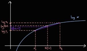

photo 2025 09 22 00 43 55 — Visualization of jensen’s inequality for log function

We then optimize to find \( q \): \[ \begin{align*} \hat{q}(z) &= \max_{q(z)} E_{z \sim q(z)} \left[ \log \frac{P(x,z;\theta)}{q(z)} \right] \\ &= \max_{q(z)} E_{z \sim q(z)} \left[ \log (P(x|z;\theta) \cdot P(z)) – \log q(z) \right] \\ &= \max_{q(z)} E_{z \sim q(z)} \left[ \log P(x|z;\theta) + \log P(z) – \log q(z) \right] \end{align*} \] Now we can, for example, apply the EM algorithm. However, there is still a challenge: we need to optimize for each data sample, which is computationally inefficient.

3.3. Amortization & Stochastic Optimization with a NN

What we derived was the traditional variational inference approach. It implies that for each data point \( \mathbf{x}_i \), we need to find the parameters that determine \( q_z \) (for example, find \( \boldsymbol{\mu} \) and \( \mathbf{C} \) in the case of a Gaussian). This leads to a slow and computationally costly process; for instance, if you have a million images, you’d need to run a million separate optimizations. The solution that was proposed in the paper “Auto-Encoding Variational Bayes” (link) is to consider an amortized variational posterior \( q_{\phi}(z|x) \) instead. Thus, instead of optimizing the parameters \( \boldsymbol{\mu} \) and \( \mathbf{C} \) for each data point \( \mathbf{x}_i \), we optimize the parameters \( \phi \) and the model outputs \( \boldsymbol{\mu} \) and \( \mathbf{C} \) for the given \( \mathbf{x}_i \), for example, using a NN with input \( \mathbf{x}_i \), parameters \( \phi \), and output \( \boldsymbol{\mu} \) and \( \mathbf{C} \), as the following figure illustrates: The amortized formulation is then: \[ \begin{align*} \hat{q}_{\phi}(z|x) &= \max_{\phi} E_{z \sim q_{\phi}(z|x)}\left[ \log p(x|z;\theta) + \log p(z) – \log q(z|x;\phi) \right] \\ &= \max_{\phi} E_{z \sim q_{\phi}} \left[ \log \frac{P(x,z;\theta)}{q(z|x;\phi)} \right] \end{align*} \] This results in a faster, better regularized optimization, but the result is not as precise. It is also worth mentioning that we get the original derived expression of the ELBO that involves the posterior \( q(z|x) \). Following this approach, we obtain an auto-encoder-like model.

4. VAE

VAEs are a type of probabilistic latent model and an unsupervised learning model, similar to GMMs. While GMMs classify data points into clusters, VAEs compress high-dimensional data into a lower-dimensional latent space. In this sense, VAEs are a form of dimensionality reduction, aiming to reduce data dimensions while preserving information. Structurally, VAEs are a type of autoencoder.

4.1. VAE as Autoencoder

An autoencoder is a model that takes an input \(x\), compresses it into a lower-dimensional latent representation \(z\), and then decompresses \(z\) to produce a reconstructed version \(x’\) of \(x\). The goal is to obtain a more compact and interpretable format of the original data point. For example, a 320×320 image (102,400 pixels) can be compressed into a vector with only 1,000 entries and then reconstructed back to its original dimensions.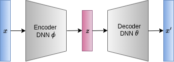

However, autoencoders can’t be used to generate new images. They are not probabilistic models, so they don’t model the data distribution. This results in an unstructured latent space, where large areas of the space do not correspond to meaningful outputs. If you sample from a nearby point \(z_1\) in the latent space, the resulting output might be either a poor reconstruction or very similar to the original image because the space lacks a smooth, continuous structure.

4.2. VAE as Probabilistic Generative Model

A VAE has the same structure as a regular autoencoder, but the key difference is that the encoder and decoder are stochastic (probabilistic). This means they represent data distributions: the encoder models the approximate posterior distribution \( q_{\phi}(z|x) \) and the decoder models the likelihood distribution \( p(x|z; \theta) \). It’s called a Variational Autoencoder because it uses an amortized variational posterior. A common example is to model both the encoder and decoder as Gaussians.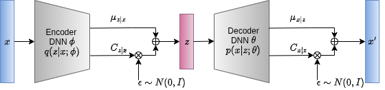

var autoencoder — VAE takes x as input. The encoder outputs the lower dimensional parameters of the modeled posterior distribution. z is sampled using the obtained parameters. The decoder gets z as input and output the parameters of distribution p(x|z). The parameters are then used to generate new samples.

To generate new samples, you first sample a point \(z\) from a standard normal distribution in the latent space. Then, you use the decoder network to map \(z\) to the parameters of the distribution \(p(x|z)\). Finally, you sample \(x\) from that parametric distribution \(p(x|z)\). The encoder is only used during the training phase, not for generation. Even though \( p(z|x) \) and \( p(x|z) \) are simple Gaussian distributions, the model can fit complicated marginal distributions \( p(x;\theta) \) because of the non-linear mapping between \(z\) and the distribution parameters. This allows for smooth transitions in the generated output as you move through the latent space:

5. Training

For training, we follow the variational inference approach to optimize the ELBO instead of the intractable log-likelihood. \[ \log P_X(x;\theta) = \sum_{i=1}^n \text{ELBO}_i + \sum_{i=1}^n D_{KL(i)}(q_{z|x}||p_{z|x}) \] Per data point ELBO: \[ L(x;\phi, \theta) = E_{z \sim q_{Z|X}(z|x)}\left[ \log \frac{P_{X,Z}(x,z;\theta)}{q_{Z|X}(z|x;\phi)} \right] \] Additionally, we adopt amortization to be able to apply stochastic optimization. With this setup, we can jointly optimize \( \phi \) and \( \theta \): 1- For \( \theta \): \[ \frac{\partial}{\partial \theta} L(x;\phi, \theta) = E_{z \sim q_{Z|X}}\left[ \frac{\partial}{\partial \theta} \log P(x,z;\theta) \right] \] \[ (\ast) \approx \frac{\partial}{\partial \theta} \log P(x,\tilde{z};\theta) \] \( (\ast) \quad \) Here we approximate the expectation with a sample \( \tilde{z} \sim q(z|x;\phi) \). More samples can be used for approximation, but practice shows that generalization performance won’t be much improved. 2- For \( \phi \): Here we have a problem, as: \[ \frac{\partial}{\partial \phi} L(x;\phi, \theta) = \frac{\partial}{\partial \phi} E_{z \sim q_{Z|X}}\left[ -\log q(z|x;\phi) \right] \] \[ \ne E_{z \sim q_{Z|X}} \left[ \frac{\partial}{\partial \phi} -\log q(z|x;\phi) \right] \] The derivation and expectation are not exchangeable. This is due to the fact that \( \phi \) appears not only in the argument of the expectation but also in the distribution used to sample \( z \) that defines the expectation operation. This can be solved with the “reparameterization trick.”

5.1. Reparameterization Trick

The reparameterization trick is a change of variable that solves the optimization of the \( \phi \) problem. We consider another random variable \( \epsilon \sim p_{\epsilon} (\epsilon) \) such that \( z = h(\epsilon,x;\phi) \sim q_{Z|X}(z|x;\phi) \). Consequently: \[ E_{z \sim q_{Z|X}(z|x;\phi)}[f(z)] = E_{\epsilon \sim p(\epsilon)}[f(h(\epsilon, x;\phi))] \] and the optimization is now possible: \[ \frac{\partial}{\partial \phi} L(x;\phi, \theta) = E_{\epsilon \sim P_\epsilon}\left[ \frac{\partial}{\partial \phi} -\log q(z(\epsilon;\phi)|x;\phi) \right] \] \[ (\ast) \approx -\frac{\partial}{\partial \phi} \log q(\tilde{z}|x;\phi) \] \( (\ast) \quad \) Again, one sample \( \tilde{z} \) is used to approximate the expectation.

5.2. VAE ELBO

Now we can define the loss function for the training, which is the sum over \( N \) (the size of the dataset) of the per-sample computed ELBO. The final simplified ELBO is derived as follows: \[ \begin{align*} L(x;\phi, \theta) &= E_{z \sim q_{Z|X}(z|x;\phi)} \left[ \log \frac{P_{X|Z}(x,z;\theta)}{q_{Z|X}(z|x;\phi)} \right] \\ &= E_{z \sim q_{Z|X}}\left[ \log p(x|z;\theta) + \log p(z;\theta) – \log q_{Z|X}(z|x;\phi) \right] \\ &= E_{z \sim q_{Z|X}}\left[ \log p(x|z;\theta) \right] – D_{KL}(q_{Z|X}||p_z) \\ &= A – B \end{align*} \] A: use one sample for approximation: \[ \begin{align*} \log p(x|z;\theta) &= \log\left( \frac{1}{\sqrt{\det(2\pi P_{C_{X|Z}})}} \exp\left(-\frac{1}{2}(x – \mu_{X|Z})^T C_{X|Z}^{-1}(x – \mu_{X|Z})\right) \right) \\ &= -\frac{d}{2}\log 2\pi – \frac{1}{2}\log \det C_{X|Z} – \frac{1}{2}(x – \mu_{X|Z})^T C_{X|Z}^{-1}(x – \mu_{X|Z}) \end{align*} \] B: \[ D_{KL}(q_{Z|X}||p_Z) = E_{z \sim q_{Z|X}}\left[ \log\frac{q_{Z|X}(z|x;\phi)}{p_Z(z)} \right] \] \[ \begin{align*} (\ast) &= E_{z \sim q_{Z|X}}\left[ \left(-\frac{d}{2}\log 2\pi – \frac{1}{2}\log \det C_{Z|X} – \frac{1}{2}(z – \mu_{Z|X})^T C_{Z|X}^{-1}(z – \mu_{Z|X})\right) – \left(-\frac{d}{2}\log 2\pi – \frac{1}{2}\log\det I – \frac{1}{2}z^T z\right) \right] \\ &= 0, \quad \log 1 = 0 \\ &= E_{z \sim q_{Z|X}}\left[ -\frac{1}{2}\log\det C_{Z|X} \right] + E_{z \sim q_{Z|X}}\left[ -\frac{1}{2}(z – \mu_{Z|X})^T C_{Z|X}^{-1}(z – \mu_{Z|X}) \right] + E\left[\frac{1}{2}z^T z\right] \\ &= \alpha + \beta + \gamma \end{align*} \] \(\alpha\): \[ \begin{align*} C_{Z|X} &= \text{diag } \sigma_{Z|X}^2 \quad (\text{choose to reduce computation}) \\ \implies \log(\det C_{Z|X}) &= \log\left(\prod_i \sigma_{Z|X}^2\right) = \sum_i \log \sigma_{Z|X}^2 = \mathbf{1}^T \log \sigma_{Z|X}^2 \\ \end{align*} \] where \( \mathbf{1}^T \) is a vector of ones and \( \log \sigma_{Z|X}^2 \) is a vector of log variances. \[ \implies \alpha \approx -\frac{1}{2}\mathbf{1}^T \log \sigma_{Z|X}^2 = -\mathbf{1}^T \log \sigma_{Z|X} \] \(\beta\): \[ \begin{align*} E_{z \sim q_{Z|X}}\left[ -\frac{1}{2}(z – \mu_{Z|X})^T C_{Z|X}^{-1}(z – \mu_{Z|X}) \right] &= E_{z \sim q_{Z|X}}\left[ -\frac{1}{2}\text{tr}\left[ C_{Z|X}^{-1}(z – \mu_{Z|X})(z – \mu_{Z|X})^T \right] \right] (\ast) \\ &= -\frac{1}{2} \text{tr}\left( E_{z \sim q_{Z|X}}\left[ C_{Z|X}^{-1} C_{Z|X} \right] \right) (\ast\ast) \\ &= -\frac{1}{2}\text{tr}(I) = -\frac{d}{2} \end{align*} \] \(\gamma\): \[ \begin{align*} E\left[\frac{1}{2}z^T z\right] &= \frac{1}{2}E_{z \sim q_{Z|X}}\left[ \text{tr}(zz^T) \right] \\ &= \frac{1}{2}\text{tr}\left( E_{z \sim q_{Z|X}}\left[ zz^T \right] \right) \\ &= \frac{1}{2}\text{tr}(C_{Z|X} + \mu_{Z|X} \mu_{Z|X}^T) (\ast) \\ &\approx \frac{1}{2}\mathbf{1}^T\sigma_{Z|X}^2 + \frac{1}{2}\|\mu_{Z|X}\|^2_2 \end{align*} \] \( (\ast) \) identity: \(C_X = E[xx^T] – E[x]E[x^T] \) \[ \\ \] Final loss: \[ \begin{align*} L(x;\phi, \theta) &\approx -\frac{d}{2} \log 2\pi – \frac{1}{2}\log\det C_{X|Z} – \frac{1}{2}(x – \mu_{X|Z})^T C_{X|Z}^{-1}(x – \mu_{X|Z}) \\ &- \mathbf{1}^T \log \sigma_{Z|X} – \frac{d}{2} + \frac{1}{2}\mathbf{1}^T\sigma^2_{Z|X} + \frac{1}{2}\|\mu_{Z|X}\|^2_2 \end{align*} \] where \( C_{X|Z} \) and \( \mu_{X|Z} \) are parameterized with \( \theta \) and depend on the input \( z \): \( C_{X|Z}(z;\theta), \mu_{X|Z}(z;\theta) \) and \( C_{Z|X}, \mu_{Z|X} \) are parameterized with \( \phi \) and depend on \( x \): \( C_{Z|X}(x;\phi), \mu_{Z|X}(x;\phi) \) \[ \\ \] To train the model, we follow these steps:

Sample a data point \( x \) from the dataset.
Feed \( x \) to the encoder to get: \( \mu_{z|x} (x;\phi) \) and \( C_{z|x}(x;\phi) \).
Apply the reparameterization trick: \( z = \mu_{z|x} (x;\phi) + C_{z|x}(x;\phi) \epsilon \) with \( \epsilon \sim N(0,I) \).
Feed \( z \) to the decoder to get: \( \mu_{x|z}(z;\theta) \) and \( C_{x|z}(z;\theta) \).
Compute the obtained loss function from the derivation.
Backpropagate the gradients to update \( \phi \) and \( \theta \).
Repeat until convergence.