Normalizing Flows Explained

1. Overview

1.1. What are Normalizing Flows?

Normalizing Flows are a class of probabilistic generative models that builds a complex probability distribution by passing a simple base distribution (like a standard Gaussian) through a sequence of invertible, differentiable transformations (the “flow”). The model learns the parameters of these transformations.

1.2. Original Motivation

To overcome the limitations of earlier generative models (like Variational Autoencoders or GANs) by enabling exact and tractable likelihood computation for density estimation, while maintaining efficient sampling and the ability to learn complex, high-dimensional distributions.

1.3. Relevant Papers

Dinh, Krueger, Bengio (2014) – “Neural Autoregressive Flows”/ (2014) – “Deep Generative Models with Gaussianizing Flows”: Introduced early forms of invertible transformations for deep generative models.
Rezende & Mohamed (2015) – “Variational Inference with Normalizing Flows”: Integrated flows with Variational Autoencoders (VAEs) to significantly improve the flexibility and expressiveness of the variational posteriors.
Dinh, Sohl-Dickstein, Bengio (2017) – “Density Estimation using Real NVP” (Non-Volume Preserving): Introduced a highly scalable and computationally efficient coupling-layer architecture that became foundational for modern flows.
Kingma & Dhariwal (2018) – “Glow: Generative Flow with Invertible 1×1 Convolutions”: Scaled up flows for high-resolution image generation and introduced the 1×1 convolution layer, demonstrating state-of-the-art results.

1.4. Current Status

Normalizing Flows are a rapidly evolving and active area of research in deep learning. While they have yet to fully surpass GANs or diffusion models in photorealistic image generation, they are highly valued for their exact likelihood computation, which is critical for tasks like anomaly detection, density estimation, and high-fidelity representation learning. New flow architectures and techniques (like integrating with continuous-time dynamics, i.e., continuous normalizing flows) are continually being developed.

1.5. Relevance

Flows provide a mathematically rigorous framework for exact density estimation and are central to modern Bayesian inference (as improved variational posteriors) and generative modeling. Their invertibility makes them suitable for both generating data and encoding it, offering a unique position among generative models.

1.6. Applications (Historical & Modern)

Density Estimation: Providing an accurate and flexible model of the probability distribution for complex datasets in areas like physics, finance, and climate modeling. Variational Inference (as a component): Used within Variational Autoencoders (VAEs) to create a much more expressive and accurate latent space distribution (posterior), improving the quality of the learned representations and reconstructions. Generative Modeling: Used for generating high-quality synthetic data, including images (though often superseded by GANs/Diffusion for pure visual fidelity), audio, and molecular structures. Lossless Data Compression: The exact log-likelihood can be directly related to the bitrate, allowing flows to be used for state-of-the-art lossless compression of images and other data. Anomaly Detection: By accurately estimating the true distribution, low log-likelihood scores identify data points far outside the distribution as anomalies or outliers.

2. Background: Change of Variable Formula

Suppose we have a random variable \( Z \) with known distribution \( p(z) \). We can obtain a new distribution \( p(x) \) of another random variable \( X \) by using the change of variable formula: \[ P_X(x) = P_Z(z=f^{-1}(x)) \cdot \left| \frac{\partial f^{-1}(x)}{\partial x} \right| \] This can also be written using the Jacobian determinant: \[ P_X(x) = P_Z(f^{-1}(x)) |\det J_{f^{-1}}(x)| \] with \( f \) a known bijective transformation such that \( x = f(z) \) and \( J \) the corresponding Jacobian Matrix, where \( J_{ij} = \frac{\partial f_i^{-1}(x)}{\partial x_j} \). We can further use the inverse function theorem: \[ |\det J_{f^{-1}}(x)| = |\det J_{f}(z)|^{-1} \] to get the final expression for \( P_X(x) \): \[ P_X(x) = P_Z(z = f^{-1}(x)) |\det J_f(z)|^{-1} \] The role of the Jacobian determinant is to normalize the distribution after applying the transformation \( f \) to counteract a possible change of volume caused by \( f \). This raises the question: is it possible to use this concept for generative modeling? Yes, we can start with a known distribution \( p(z) \) (a Gaussian, for example), then apply invertible transformations sequentially to obtain a flexible complex distribution \( p(x) \).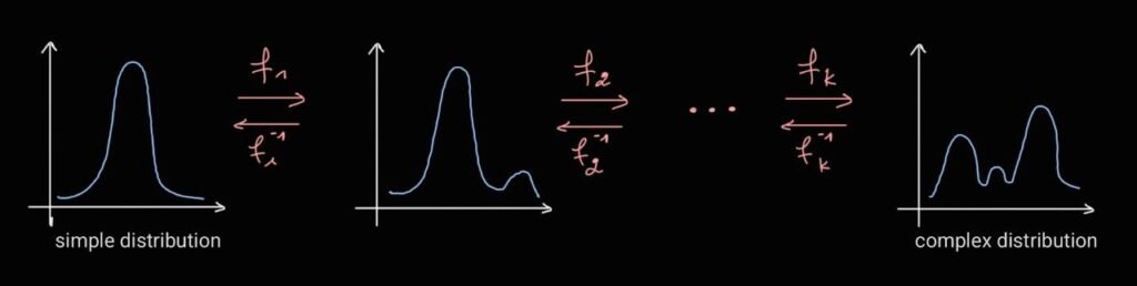

photo 2025 09 27 08 20 23 — An Example of Transforming a simple distribution to a complex distribution through a series of invertible functions.

3. The Concept of Normalizing Flows

Recall that to generate new samples based on an available dataset, in a probabilistic framework, we opt to model the likelihood function \( p(x;\theta) \). During training, we fit this likelihood to the available data by optimizing the parameters \( \theta \). Normalizing Flows (NFs) follow another approach: we learn the mapping instead of the actual distribution. The core concept of NFs is to learn an invertible (bijective) and differentiable function that maps from a simple known distribution \( p(z) \) to a complex distribution \( p(x) \). Once we pick the mapping function, we can apply the principle of the change of variables for PDFs: \[ P_X(x) = P_Z(T^{-1}(x, \theta)) |\det J_{T^{-1}}(x)| \] with \( x = T(z, \theta) \). The fact that the transformation has to be invertible implies that the latent space can’t be lower dimensional anymore. Thus, the latent space must be the same dimension as the data space, which can lead to high computational costs. This is mainly due to the evaluation of the determinant, which costs \( O(D^3) \) in the case of \( D \times D \) images as input. The resulting models consisting of invertible transformations with tractable Jacobian determinants are called Normalizing Flows or flow-based models. According to “Deep learning Foundations and concepts,” the name comes from the analogy between the sequential mappings of the probability distribution and the flow of a fluid. And “normalizing” comes from the effect of the inverse mappings, which transform the complex distribution \( p(x) \) into a normalized form \( p(z) \).

4. Difference between NFs and VAEs

In VAEs, we highlighted that we can’t work directly with the likelihood function because it is intractable when working with a continuous latent space. The solution was to approximate it using the ELBO based on the variational inference approach. NFs opt to restrict the form of the neural network such that the likelihood function can be evaluated without approximation. On the other hand, in contrast to VAEs, NFs do not optimize the likelihood function explicitly. When the training is done, we do not have access to the likelihood function to sample from; instead, we sample using the known PDF \( p(z) \) and the learned transformation \( T \). That’s why VAEs are referred to as prescribed models, while NFs are categorized as implicit probabilistic generative models.

5. The NFs Model

The structure is motivated by the way we model the invertible mapping as well as the ease of training. This mapping needs to be flexible to obtain a complex distribution \( p(x) \) that models a wide range of distributions and is easy to parametrize and train. To this end, we use invertible neural networks, which means all layers are invertible. The transformation \( T \) will then be a concatenation of transformations: \( T = T_K \circ T_{K-1} \circ \dots \circ T_1 \), where each \( T_j \) is modeled by an invertible NN with parameters \( \theta \). illustrates the structure of NFs.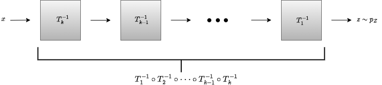

NFs — Illustration of the Normalizing Flows Model’s structure

To learn the underlying distribution of the data, we optimize the parameters \( \theta \) with respect to the Maximum Likelihood Estimation principle as usual: \[ \begin{align*} \max_{\theta} \log P_X(x) &= \max_{\theta} \sum_{i=1}^n \log P_X(x_i) \\ &= \max_{\theta} \sum_{i=1}^n \left[ \log P_Z(T^{-1}(x_i, \theta)) + \log |\det J_{T^{-1}}(x_i)| \right] \\ (\ast) &= \max_{\theta} \sum_{i=1}^n \left[ \log P_Z(T^{-1}(x_i, \theta)) + \log \prod_{j=1}^K |\det J_{T_j^{-1}}(g_j(x_i))| \right] \\ &= \max_{\theta} \sum_{i=1}^n \left[ \log P_Z(T^{-1}(x_i, \theta)) + \sum_{j=1}^K \log |\det J_{T_j^{-1}}(g_j(x_i))| \right] \end{align*} \] with \( g_j(x) = (T_{j+n}^{-1} \circ \dots \circ T_{K}^{-1})(x) \) the concatenation of \( K \) transformations \( T_j \). \( (\ast) \quad \) This rule is for the concatenation of transformations. It is a generalization of a single concatenation: \[ \det J_{T_2 \circ T_1}(x) = \det J_{T_2}(T_1(x)) \cdot \det J_{T_1}(x) \]

6. Coupling Flows

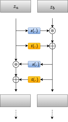
How do we design the model such that the NNs are invertible? How do we make sure that calculating the Jacobian determinants is computationally feasible to be able to train the model? This section answers these two questions. RealNVP (Real-valued Non-Volume Preserving flows) is a normalizing flow model proposed by Dinh et al. in 2016. The concept is to divide the latent variable vector \( z \) into two parts: \( z = [z_a, z_b] \). For example, \( z_a = z_{1:d} \) and \( z_b = z_{d+1:D} \) (keep in mind that \( x \) and \( z \) must have the same dimension \( D \) for invertibility). Accordingly, we partition the vector \( x = [x_a, x_b] \) with corresponding dimensions \( d \) and \( D-d \). The transformation \( T \) is then defined as follows: \[ \begin{cases} x_a = z_a \\ x_b = \exp(s(z_a, \theta)) \odot z_b + t(z_a, \theta) \end{cases} \] where \( s(\cdot) \) and \( t(\cdot) \) are Neural Networks with parameters \( \theta \), and \( \odot \) is the Hadamard product for elementwise multiplication.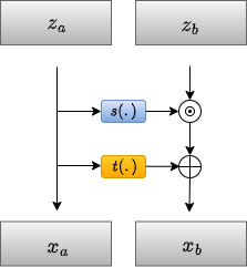

CNFs — A single layer of the real NVP normalizing layer. s(.) and t(.) are two neural networks that will be trained.

This design of the transformation is invertible by definition. The inverse transformation \( T^{-1} \) is: \[ \begin{cases} z_a = x_a \\ z_b = (x_b – t(x_a, \theta)) \odot \exp(-s(x_a, \theta)) \end{cases} \] On the other hand, the determinant can be efficiently calculated as this model results in the following Jacobian matrix: \[ J = \begin{bmatrix} I_{d} & O_{d \times (D-d)} \\ \frac{\partial z_b}{\partial x_a} & \text{diag}(\exp(-s)) \end{bmatrix} \] \( I_d \) is a consequence of \( z_a = x_a \), while \( O_{d \times (D-d)} \) is because \( z_a \) is independent of \( x_b \). The second line contains the derivatives of \( z_b \) with respect to \( x \). We can see that the Jacobian matrix is a lower triangular matrix; thus, the determinant is just the product of the diagonal elements. The determinant is given by: \[ \det(J) = \prod_{j=1}^{D-d} \exp(-s_j(z_a, \theta)) \] As illustrates, we can use two neural networks, \( s(\cdot) \) and \( t(\cdot) \), for scaling and shifting/translation respectively. This results in a very flexible output \( x_b \). However, we can see that we process only half of the input each time—that is, the value of \( z_a \) is never changed. To solve this problem, we alternate between the partitions such that the whole input is affected by the transformation, as shown in the figure.