Generative Adversarial Networks Explained

1. Overview

1.1. What are Generative Adversarial Networks (GANs)?

Generative Adversarial Networks GANs are a class of generative models that learns to produce new data instances with the same characteristics as the training data through a game-theoretic scenario (a minimax game) between two competing neural networks: a generator and a discriminator.

1.2. Original Motivation

Designed to overcome the difficulties of training traditional generative models (like earlier Variational Autoencoders or Boltzmann Machines) by replacing explicit density function calculation with a competition. This made it possible to generate high-fidelity, realistic samples (especially images) that were previously unattainable.

1.3. Relevant Papers

Ian Goodfellow et al. (2014) – “Generative Adversarial Nets”: Introduced the concept of GANs, the objective function (the minimax game), and demonstrated the ability to generate simple images.
Alec Radford, Luke Metz, Soumith Chintala (2015) – “Unsupervised Representation Learning with Deep Convolutional Generative Adversarial Networks (DCGAN)”: Standardized the architecture by using Convolutional Neural Networks (CNNs) for both the generator and discriminator, which significantly improved the stability and quality of image generation.

1.4. Current Status

GANs are one of the most active and successful areas of research in deep learning. They continue to push the state-of-the-art in image and video generation, but research also focuses heavily on improving training stability (a key challenge) and mitigating common issues like mode collapse.

1.5. Relevance

GANs are highly relevant as they provide an effective framework for unsupervised and semi-supervised learning, particularly in tasks requiring the creation of high-dimensional, realistic, and novel data. They have had a transformative impact on the fields of computer vision and creative AI.

1.6. Applications (Historical & Modern)

Image Synthesis: Creating photorealistic images, translating images from one domain to another (CycleGAN), super-resolution, and image-to-image translation (e.g., changing weather in a photo). Data Augmentation: Generating synthetic, yet realistic, samples to expand limited datasets for tasks like classification. Computer Graphics & Entertainment: Generating new textures, faces, and creating deepfakes (a controversial application). Drug Discovery & Materials Science: Designing novel molecular structures with desired properties.

2. From Probabilistic Modeling to Deep Learning

2.1. The General Approach So Far

The three models we have seen so far—GMMs, VAEs, and NFs—follow a probabilistic modeling approach. The learning of the data distribution is guided by the log-likelihood as a loss function and Maximum Likelihood Estimation (MLE) as a probabilistic approach. For this approach to work, we had to make many assumptions:

VAEs: latent variable structure, specific forms of the likelihood (ELBO) and variational posterior (Gaussian) density networks.
NFs: functions must be invertible and Jacobian determinant evaluation must be computationally feasible. As we have seen in the last post, this limits the structure of the mapping network.

A fair question is: Can we model the data better by having fewer assumptions? Idea: given initial noise \( z \sim \mathcal{N}(0,I) \), is it possible to use a flexible function to transform the noise \( z \) into the target data space \( x \sim p(x) \) using a transformation (mapping) \( f_{\theta}(z) \)? In contrast to NFs, the transformation can be any function.

2.2. Generative Adversarial Networks (GANs) Concept

When we transitioned from GMMs to VAEs and then to NFs, the amount of reliance on Deep Learning (DL) increased. GANs represent a pure deep learning approach. Instead of a model that learns a closed-form (GMMs, NFs) or approximate (VAEs) formula of the probability density function of the data, GANs totally rely on DL to model the data by training two networks:

Generator (G): takes noise as input and outputs a fake sample.
Discriminator (D): receives samples from both the generator and training data and has to distinguish between the two by classifying the input as “real” or “fake”.

The goal is to train the generator in such a way that the discriminator cannot distinguish between real and “fake” samples. GANs are named so because of the Game-Theoretic scenario between the two competing networks G and D. The GAN framework is based on a non-cooperative and zero-sum game between G and D. It is worth mentioning that although GANs rely on deep learning for modeling data, they implicitly model the likelihood, as will be shown in section 4. In this context, GANs are considered implicit probabilistic generative models, similar to NFs. Thus, for sampling, we discard the discriminator because it is only used for training, and we give an input \( z \sim \mathcal{N}(0,I) \) to the generator to get a sample \( x_{\text{sample}} \) as output, but we do not have access to the likelihood function itself.

3. GANs Structure and Adversarial Training

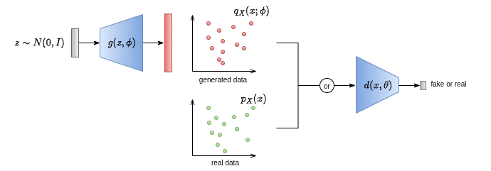
As already mentioned, the Generator and the Discriminator are parameterized using deep neural networks:

Generator: \( g(z,\phi) \) maps noise \( z \sim p_Z \) to a sample \( x \sim p_X \).
Discriminator: \( d(x,\theta) \) is a classifier that outputs an estimate of the posterior probability \( p(Y_i = 1 | x_i) \sim d(x_i,\theta) \), where:
- \( Y_i = 1 \) when \( x_i \in D \) (\( x_i \) is real)
- \( Y_i = 0 \) when \( x_i = g(z,\phi) \) (\( x_i \) is fake)

This results in the following posterior expression: \[ p(Y_i|x_i;\theta) = d(x_i,\theta)^{Y_i} (1-d(x_i,\theta))^{1-Y_i} \] Now, the adversarial loss can be derived as follows: First, we train the discriminator, which corresponds to a Maximum A Posteriori (MAP) estimation problem: \[ \max_{\theta} \sum_i \log p(Y_i|x_i;\theta) = \max_{\theta} \sum_i \log d(x_i,\theta)^{Y_i} (1-d(x_i,\theta))^{1-Y_i} \] \[ = \max_{\theta} \sum_i \left( Y_i \log d(x_i,\theta) + (1-Y_i) \log (1-d(x_i,\theta)) \right) \] Then, consider the generator (where \( x_i \) is replaced by a fake sample \( g(z_i, \phi) \), making \( Y_i = 0 \)): \[ \max_{\theta} \sum_i \left( Y_i \log d(x_i,\theta) + (1-Y_i) \log (1-d(g(z_i,\phi),\theta)) \right) \] Finally, the goal of adversarial training is defined by the **minimax game** between the generator and the discriminator: \[ \min_{\phi} \max_{\theta} L_{\text{GAN}} \] \[ \min_{\phi} \max_{\theta} \sum_i \left( \log d(x_i,\theta) + \log (1-d(g(z_i,\phi),\theta)) \right) \] where \( Y_i \) is now implicit. For example:

If \( x_i \) is a real sample from the dataset, then we consider only the first term:
- If \( d \sim 1 \) (guessed correctly) then \( L_{\text{GAN}} \sim 0 \) (small loss) because of the log.
- If \( d \sim 0 \) (wrong guess) then \( L_{\text{GAN}} \to -\infty \) (large loss).
If \( x_i \) is fake (generated by \( g \)), then only the second term is considered:
- If \( d \sim 1 \) (guessed correctly) then \( L_{\text{GAN}} \to -\infty \) (large loss).
- If \( d \sim 0 \) (wrong guess) then \( L_{\text{GAN}} \sim 0 \) (small loss).

From the loss expression, we can see that the discriminator \( d \) is trained to minimize the loss (which corresponds to \( \max_{\theta} \)), while the generator \( g \) is trained to maximize the loss (which corresponds to \( \min_{\phi} \)). If \( g \) could find perfect weights \( \phi \), then \( d \) can’t tell the difference between fake and real samples, and the loss will converge to \( 0.5 \). For more insight, the loss can be expressed as the expectation over the data and noise distributions: \[ L_{\text{GAN}} = \frac{1}{N_{\text{real}}} \sum_{i=1}^{N_{\text{real}}} \log d(x_i, \theta) + \frac{1}{N_{\text{fake}}} \sum_{i=1}^{N_{\text{fake}}} \log (1 – d(g(z_i, \phi), \theta)) \]

4. Adversarial Training as a Minimization of the JS Divergence

After deriving the optimization problem of GANs, we can delve deeper into why the minimax approach of adversarial training can lead to obtaining a generative model. We start by examining the true error in the min-max optimization problem: \[ \min_{\phi} \max_{\theta} \left\{ E_{x \sim P_X} \left[ \log d(x, \theta) \right] + E_{z \sim P_Z} \left[ \log (1 – d(g(z, \phi), \theta)) \right] \right\} \] Recall that during training, the expectation will be approximated using the training dataset \( D=\{x_i\}_{i=1}^n \) and \( n \) samples from the latent variable distribution \( p_Z \), also referred to as noise. Then, we look for the optimal solution of this optimization problem to understand what we are trying to reach theoretically. First, we derive the optimal discriminator \( \hat{d} \) for a given generator \( g \) (we fix \( g \) or fix its parameters) that generates samples from a distribution \( q_X(x;\phi) \): \[ \max_{\theta} E_{x \sim P_X}[\log d(x, \theta)] + E_{x \sim q_X}[\log (1 – d(x, \theta))] \] \[ \begin{align*} (\ast) &= \max_{\theta} \left\{ \int_x P_X(x) \log d(x, \theta) \,dx + \int_x q_X(x) \log (1 – d(x, \theta)) \,dx \right\} \\ &= \max_{\theta} \int_x \left[ P_X(x) \log d(x, \theta) + q_X(x;\phi) \log (1 – d(x, \theta)) \right] \,dx \end{align*} \] Here we can maximize the term inside the integral. A pointwise maximization of the integrand is convex: \[ \frac{\partial}{\partial d(x, \theta)} \left[ P_X(x) \log d(x, \theta) + q_X(x;\phi) \log (1 – d(x, \theta)) \right] \stackrel{!}{=} 0 \] \[ \implies \frac{P_X(x)}{d(x, \theta)} – \frac{q_X(x;\phi)}{1 – d(x, \theta)} \stackrel{!}{=} 0 \] Solving for \( d(x, \theta) \) gives the optimal discriminator function: \[ \hat{d}(x) = \frac{P_X(x)}{P_X(x) + q_X(x;\phi)} \] \( (\ast) \quad E_{x \sim f(x)} [g(x)] = \int_x f(x) \cdot g(x) \,dx \) Next, we proceed with the optimal generator \( \hat{g} \) given the optimal discriminator \( \hat{d} \): \[ \min_{\phi} E_{x \sim P_X}\left[ \log\left( \frac{P_X(x)}{P_X(x) + q_X(x;\phi)} \right) \right] + E_{x \sim q_X}\left[ \log\left( \frac{q_X(x;\phi)}{P_X(x) + q_X(x;\phi)} \right) \right] \] \[ \begin{align*} &= \int_x \left[ P_X(x) \log\left( \frac{2P_X(x)}{P_X(x) + q_X(x;\phi)} \right) + q_X(x;\phi) \log\left( \frac{2q_X(x;\phi)}{P_X(x) + q_X(x;\phi)} \right) \right] – \log 4 \,dx \\ &= D_{KL}(P_X(x)||m(x)) + D_{KL}(q_X(x;\phi)||m(x)) – \log 4, \quad \text{with } m = \frac{1}{2}(P_X(x) + q_X(x;\phi)) \\ &= \min_{\phi} 2 D_{JS}(P_X(x)||q_X(x;\phi)) – \log 4, \quad \text{with } D_{JS} \text{ the } \textbf{Jensen-Shannon divergence} \end{align*} \] We conclude that training GANs is equivalent to minimizing the JS divergence \( D_{JS} \) between \( p_X \) (the true data distribution) and \( q_X(x;\phi) \) (the approximate distribution). The optimal generator \( g \) corresponds to the minimal \( D_{JS}(p_X||q_X)=0 \), which is equivalent to a minimal loss \( L_{\text{GAN}} = -\log 4 \).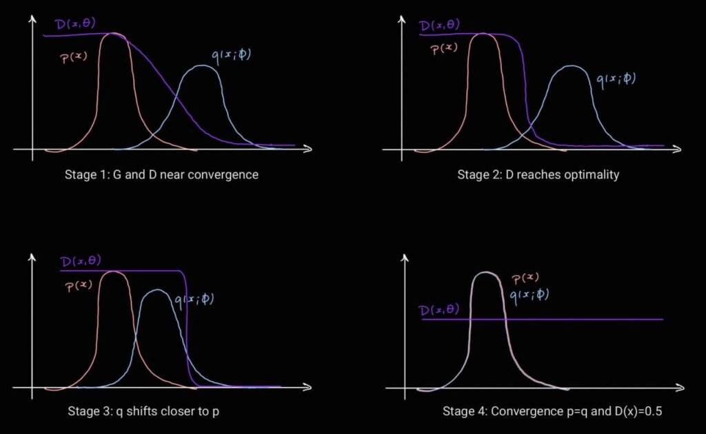

photo 2025 10 04 06 39 46 — A schematic representation of how the adversarial training is intended to be

5. GANs Limitations

5.1. Optimal Discriminator

This issue happens usually at the beginning of the training. The discriminator is almost optimal at this stage, and the fake samples from the generator are easily detectable. This results in vanishing gradients with respect to the generator’s parameters \( \phi \), and thus the generator can’t learn or improve. We can also see this from the JS divergence perspective, as derived for the optimal generator in the previous section. Easily detectable generated samples are equivalent to non-overlapping \( p_X(x) \) and \( q_X(x;\phi) \). This makes \( D_{JS} (p_X||q_X)=\log(2) \), which is the maximum value when the base of the logarithm is 2. This results in a constant objective with a zero gradient during the Generator optimization. For more intuition, we can visually understand it in the second stage from the GAN training figure. If the supports of \( p_X(x) \) and \( q_X(x;\phi) \) do not overlap, the transition of the discriminator curve from 1 to 0 will be steeper and look more like a step function. When the generator updates its parameters to shift its distribution, the change will be minimal or negligible, and as a result, the gradient (which measures how much variation happened) vanishes. More powerful variations of GANs were invented to avoid this issue, for example, the Wasserstein GAN (WGAN). It uses the Wasserstein-1 distance in the loss function that guarantees a smoother measure of the supports’ distance.

5.2. Lazy Discriminator and Mode Collapse

This is the opposite situation of the previous issue. If the Generator (G) is too good (e.g., updates faster than the Discriminator (D)), D cannot provide useful feedback to G because it is too confused. This leads to the problem of mode collapse, where G produces only one or two specific high-quality samples that D can’t distinguish. Common solutions for this problem include increasing the updating steps \( k \) of D for each step of G, controlling the learning rates such that \( \text{lr}(D) > \text{lr}(G) \), or using minibatch discrimination, where we give D information about other samples to detect if the same or similar samples are always generated.

5.3. Non-Convergence

This issue is due to the min-max optimization, which does not converge always. The objective increases if G improves and decreases if D gets better. This leads to an oscillatory behavior and makes selecting the step size and determining the convergence of training challenging.