Gaussian Mixture Models Explained

1. Overview

1.1. What are Gaussian Mixture Models?

Gaussian Mixture Models are probabilistic models that expresse a probability distribution as a combination of multiple Gaussian (normal) distributions, each contributing with a certain weight.

1.2. Original Motivation

Designed to capture heterogeneous or multi-modal data by breaking down a complex distribution into simpler, interpretable Gaussian components.

1.3. Relevant Papers

1. Karl Pearson (1894): Early work on fitting mixtures of normal distributions.
2. Dempster, Laird, Rubin (1977) – “Maximum Likelihood from Incomplete Data via the EM Algorithm”: Introduced the EM algorithm, which made maximum-likelihood estimation of mixture models computationally feasible and remains the standard fitting approach.
3. Duda & Hart (1973): Their textbook spread the use of GMMs in clustering and classification.

1.4. Current Status

GMMs are still extensively applied and continuously supported in modern statistics and machine learning libraries (such as R and Python). Ongoing research continues to refine methodology and applications.

1.5. Relevance

Although deep learning has overtaken GMMs in areas like large-scale speech recognition, they remain valuable as interpretable, efficient, and lightweight models for density estimation, clustering, and as components in larger ML pipelines.

1.6. Applications (Historical & Modern)

Speech recognition: Before deep learning, GMM–HMM systems were the backbone of acoustic modeling.

Computer vision: Widely used for background subtraction and motion detection through pixelwise Gaussian mixtures.

General clustering & density modeling: Found in diverse scientific and engineering domains such as biomedical imaging, astronomy, and anomaly detection.

2. Probabilistic Modeling with GMMs for Clustering

GMMs (Gaussian Mixture Models) are popular for data clustering.

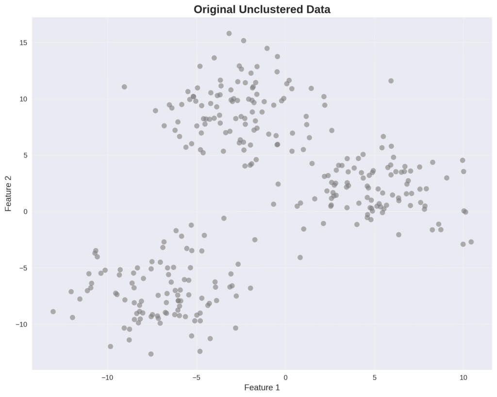
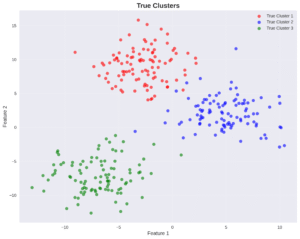
2.1. What is Clustering?

Clustering is a form of unsupervised learning. The goal is to divide multi-dimensional data into clusters, or groups of data points. While this post series is about the task of generating data, understanding data clustering can be very helpful. The main reason is because it demonstrates the importance of probabilistic modeling, as we will see when comparing the K-means algorithm and GMMs for clustering.

2.2. K-Means Clustering

An iterative algorithm used for clustering (not probabilistic).

Suppose we have a dataset \( \mathbf{x} = \{\mathbf{x}_1,…,\mathbf{x}_N\} \), the number of observations \( N \), and the dimension of the data (each sample \( \mathbf{x}_i \)) is \( D \). The goal is to divide the data into \( K \) clusters. For that, the K-means algorithm introduces \( K \) vectors \( \boldsymbol{\mu}_k \) with dimensionality \( D \), where each vector \( \boldsymbol{\mu}_k \) represents the mean of cluster \( k \).

The algorithm then finds those \( \boldsymbol{\mu}_k \) and the associated data points such that the distance of each data point to the corresponding mean \( \boldsymbol{\mu}_k \) is minimal. The association is determined through a parameter \( r_{ik} \in \{0,1\} \), where \( r_{ik} \) is equal to 1 only for the selected cluster, otherwise it is 0. The parameters \( \boldsymbol{\mu}_k \) and \( r_{ik} \) are found by solving this optimization problem:

\[ (r,m) = \arg \min_{r,m} \sum_{i}^{n} \sum_{k}^{K} r_{ik}\|\mathbf{x}_i – \mathbf{m}_k\|^2 \]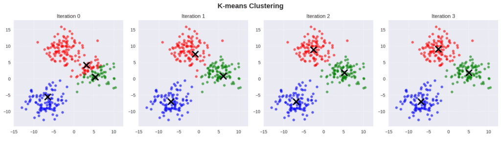

2.3. Mixture Models

Simplest form of latent variable models (probabilistic).

We assume there are \( K \) Gaussian components that, combined, determine the distribution of the data \( \mathbf{X} \). There is a discrete latent random variable \( Z \) with realizations \( z \in \{1,2,…,K\} \), where each value \( z \) corresponds to a component of the mixture model. This latent variable simply states that the sample \( \mathbf{x}_i \) belongs to the cluster \( k \).

As discussed in post 1, we use probability for modeling, so we consider \( P(z=k) \) to be the probability of picking the \( k \)-th component. These are also the weights: the contribution of each component to the mixture. \( \sum P(z=k) = 1 \).

Each component can be a different model, for example, a Gaussian or a Bernoulli. Each model has learnable parameters that define the distribution, for example, \( \boldsymbol{\mu} \) and \( \boldsymbol{\Sigma} \) in the case of a Gaussian or \( p \) (probability of success) in the case of a Bernoulli.

From a probabilistic perspective, a cluster corresponds to a mixture component. The data distribution is a mixture (summation) of models. Mixture models are represented by the following equation:

\[ p(\mathbf{x}_i|\boldsymbol{\theta}) = \sum_{k=1}^{K} p_Z(\mathbf{k}) p_{X|Z}(\mathbf{x}_i|\mathbf{k},\boldsymbol{\theta}) \]

\( \boldsymbol{\theta} \) are the learned parameters. \( K \) is a hyperparameter indicating the estimated number of clusters (not learned).

\( P(\mathbf{x}|z) \) is the probability of observing \( \mathbf{x} \) given that it was generated from a specific component \( k \) for \( z=k \).

2.4. GMMs

GMMs use the multivariate Gaussian distribution as a model:

\[ f_{\mathbf{X}}(x_1, \dots, x_k) = \frac{\exp\left(-\frac{1}{2}(\mathbf{x}-\boldsymbol{\mu})^{\text{T}}\boldsymbol{\Sigma}^{-1}(\mathbf{x}-\boldsymbol{\mu})\right)}{\sqrt{(2\pi)^k|\boldsymbol{\Sigma}|}} \]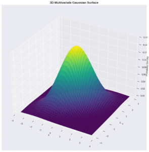

The corresponding equation is:

\[ p(\mathbf{x}_i|\boldsymbol{\theta}) = \sum_{k=1}^{K} p_Z(\mathbf{k}) \mathcal{N}(\mathbf{x}_i|\boldsymbol{\mu}_k, \boldsymbol{\Sigma}_k) \]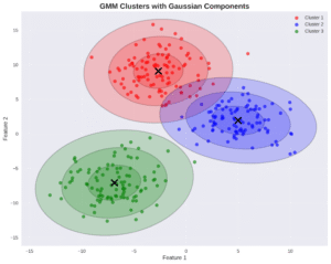

Now, to simplify notation, \( \theta = \{\mu, \Sigma, \pi\} \). Those are the learnable parameters.

2.5. Transition from K-Means to GMM and Role of Probabilistic Modeling

In this context, GMMs are probabilistic models usually presented as a generalization of the K-means algorithm. The fact that K-means is not probabilistic makes the resulting clusters unintuitive and in many cases wrong. That’s why K-means is considered a rigid clustering method while GMMs allow for soft clustering by adding variance to the equation, as shown in the equation below.

The corresponding equation is: \[ p(\mathbf{x}_i|\boldsymbol{\theta}) = \sum_{k=1}^{K} p_Z(\mathbf{k}) \mathcal{N}(\mathbf{x}_i|\boldsymbol{\mu}_k, \boldsymbol{\Sigma}_k) \]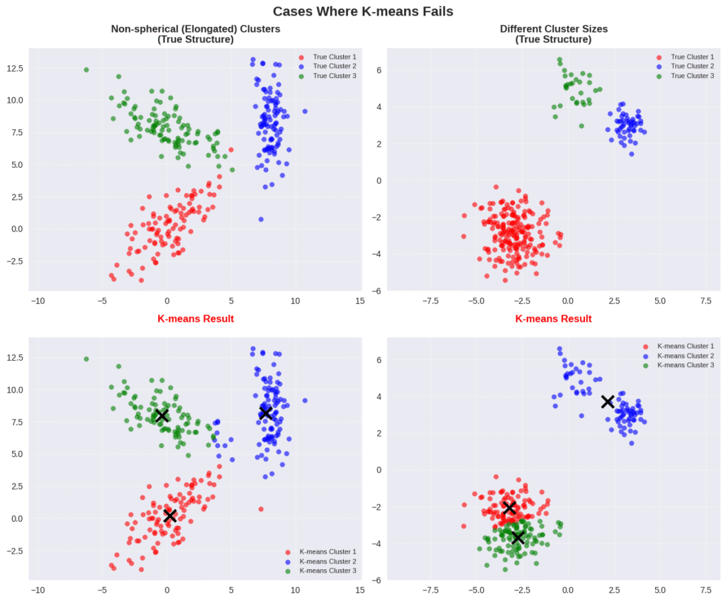

The mathematical derivation of the transition from K-means to GMM by including a parameter for variance is as follows:

\[ \begin{align*} (r,m) &= \arg \min_{r,m} \sum_{i}^{n} \sum_{k}^{K} r_{ik}\|\mathbf{x}_i – \mathbf{m}_k\|^2 \\ &= \arg \max_{r,m} \sum_{i}^{n} \sum_{k}^{K} r_{ik}(-1/2\sigma^{-2}\|\mathbf{x}_i – \mathbf{m}_k\|^2) + \text{const.} \\ &= \arg \max_{r,m} \prod_{i} \sum_{k} r_{ik} \exp (-1/2\sigma^{-2}\|\mathbf{x}_i – \mathbf{m}_k\|^2) /Z \\ &= \arg \max_{r,m} \prod_{i} \sum_{k} r_{ik}\mathcal{N}(\mathbf{x}_i; \mathbf{m}_k, \sigma^2I) \\ &= \arg \max_{r,m} p(\mathbf{x}|\mathbf{m}, r) \end{align*} \]

Line 2: We added a minus sign to go from minimization to maximization, then multiplied by a constant \( \sigma \), which does not change the solution (the location of the maximum). The const. term represents any parts of the Gaussian PDF that do not depend on \( (r,m) \). It is better understood when going backward from the next steps; for example, \( \text{const.} = -1/2 \log(2\pi\sigma^2) \).

Line 3: The sum over \( i \) becomes a product (\( \prod_i \)) when we take the exponent of the entire sum. This is based on the identity \( e^{a+b} = e^a \cdot e^b \). \( Z^{-1} \) represents the normalization constant from the Gaussian PDF.

The derivation shows that a minimization of empirical risk (a machine learning term for the risk evaluated for training instead of the unavailable true risk) corresponds to the maximization of likelihood. This is an important point to note because most probabilistic generative models maximize the log-likelihood for learning (during training).

The derivation highlights the importance of probabilistic modeling: it shows that K-means tries to maximize the likelihood of the data only in terms of the means. Thus, K-means ignores the variance parameter \( \sigma \), which defines the scale or shape of the cluster.

K-means is equivalent to GMMs if we only consider isotropic Gaussians (where variance is constant). However, excluding \( \sigma \) from the optimization makes the algorithm unable to adapt to different shapes. In terms of generation tasks, by ignoring \( \sigma \), we are not able to draw from a Gaussian distribution as a representation of data.

In other words, we do not truly understand what the clusters actually mean. So, K-means implicitly assumes that the clusters have a Gaussian shape, but it does not give us access to the parameters necessary to adapt to shapes other than a circle.

3. GMMs as Generative Models

3.1. Training

While GMMs are popular for clustering, they can also be used as generative models.

In probabilistic generative modeling, we look for the likelihood of the data, which is given by the mixture of Gaussians formula, as explained in the previous section.

We need to optimize the parameters \( \Theta \) of the model so that it can fit the data; in other words, we need to learn the data distribution. We do that by maximizing the log-likelihood function, following the MLE principle discussed in the previous post. We solve this optimization problem:

\[ \hat{\Theta} := \arg \max_{\Theta} \prod_{i=1}^{n} p(\mathbf{x}_i; \Theta) \]

Again, the log-likelihood tells us how likely it is to observe the data for given parameters \( \Theta \). Thus, when we solve the optimization problem, we should have a GMM with parameters \( \Theta \) that models the distribution \( p(\mathbf{x}; \Theta) \) and is capable of generating or drawing samples from that distribution. The question now is: How do we solve this optimization problem numerically?

To achieve that, there are two options:

• EM Algorithm: a standard classical approach
• Gradient-based approach

We first start by explaining the algorithm generally, then we apply it to GMMs. The second approach is more straightforward. We just need to calculate the gradient of the log-likelihood with respect to the parameters and then update the parameters.

3.1.1 Expectation-Maximization (EM) Algorithm

This is a powerful iterative method for finding maximum likelihood estimates for latent variable models. In these models, the log-likelihood is formulated by marginalizing out the latent variables:

\[ \begin{cases} P(\mathbf{x};\Theta) = \sum_{z} P_{Z}(z) P_{X|Z}(\mathbf{x}|z; \Theta) \quad (\text{discrete}) \\ P(\mathbf{x};\Theta) = \int_{Z} P_{Z}(z) P_{X|Z}(\mathbf{x}|z; \Theta) \,dz \quad (\text{continuous}) \end{cases} \]

Problem: It is generally hard to directly maximize the log-likelihood analytically because of the integral or sum involved in the log-likelihood expression. The logarithm over a sum or integral makes it hard to calculate the derivative of that expression and find a closed-form solution.

Solution: The EM algorithm involves two steps to solve this maximization problem:

E-step (Expectation):

In this step, we use the current model parameters \( (\Theta_t) \) to compute the posterior probabilities \( p(Z|\mathbf{X},\Theta_t) \). These probabilities tell us the likelihood of each data point belonging to a particular latent state or cluster. Using these probabilities, we then define the Q-function, which is the expected value of the complete-data log-likelihood.

\[ Q_{t}(\Theta) = E_{z \sim p(z|x; \Theta_t)}\left[ \log P_{X,Z}(\mathbf{x},z; \Theta) \right] \] The Q-function is represented by two cases: \[ \begin{cases} \sum_{z} P_{Z|X}(z|\mathbf{x}; \Theta_t) \log P_{X,Z}(\mathbf{x},z; \Theta), & \text{discrete} \\ \int P_{Z|X}(z|\mathbf{x}; \Theta_t) \log P_{X,Z}(\mathbf{x},z; \Theta) \,dz, & \text{continuous} \end{cases} \]

For that, we obviously need a model that allows us to calculate the posterior \( p(z|\mathbf{x}; \Theta_t) \). Keep in mind that the Q-function includes two “versions” of \( \Theta \): one is old, \( \Theta_t \), corresponding to the previous iteration, and one is new, \( \Theta \), evaluated at the current iteration.

M-step (Maximization):

In this step, we take the Q-function and maximize it with respect to the new parameters \( (\Theta) \). This maximization is typically a convex optimization problem with a closed-form solution, making it straightforward to solve. The resulting values become our updated parameters, \( \Theta_{t+1} \).

\[ \Theta_{t+1} = \arg \max_{\Theta} Q_t(\Theta) \]

The algorithm repeats these two steps until the parameters converge ( \( |\Theta_{t+1} – \Theta_t| \) is small enough). At this point, a local maximum of the original log-likelihood is found.

The EM algorithm solves the optimization problem by following an alternating optimization approach using the Q-function instead of the log-likelihood. In the Q-function, we flip the log and the integral, which is easier to work with. But why the Q-function? See the next post…

3.1.2 MLE for GMM using EM Algorithm

Derivation of the E-Step: formulate the Q-Function:

\[ \begin{align*} Q_t(\Theta) &= \sum_{i=1}^n E_{z_i \sim P_{Z|X}(z_i|\mathbf{x}_i; \Theta_t)}\left[ \log P_{X,Z}(\mathbf{x}_i, z_i; \Theta) \right] \\ &= \sum_{i=1}^n \sum_{k=1}^K P_{Z|X}(z_i=k | \mathbf{x}_i; \Theta_t) \log P_{X,Z}(\mathbf{x}_i, z_i=k; \Theta) \end{align*} \] \[ \begin{align*} \log P_{X,Z}(\mathbf{x}_i, z_i=k; \Theta) &= \log\left( P_{Z}(k) \cdot P_{X|Z}(\mathbf{x}_i | z_i=k; \Theta) \right) \\ &= \log P_Z(k) + \log\left( \mathcal{N}(\mathbf{x}_i | \boldsymbol{\mu}_x(k), \mathbf{C}_x(k)) \right) \\ &= \log P_Z(k) – \frac{d}{2}\log(2\pi) – \frac{1}{2}\log\det(\mathbf{C}_x(k)) – \frac{1}{2}(\mathbf{x}_i – \boldsymbol{\mu}_x(k))^T \mathbf{C}_x(k)^{-1}(\mathbf{x}_i – \boldsymbol{\mu}_x(k)) \end{align*} \] \[ Q_t(\Theta) = \sum_{i=1}^n \sum_{k=1}^K P_{Z|X}(z_i=k | \mathbf{x}_i; \Theta_t) \left[ \log P_Z(k) – \frac{d}{2}\log(2\pi) – \frac{1}{2}\log\det(\mathbf{C}_x(k)) – \frac{1}{2}(\mathbf{x}_i – \boldsymbol{\mu}_x(k))^T \mathbf{C}_x(k)^{-1}(\mathbf{x}_i – \boldsymbol{\mu}_x(k)) \right] \]

Derivation of the M-Step: find \( \Theta \) that maximizes \( Q_t(\Theta) \):

\[ \Theta_{t+1} = \arg \max_{\Theta} Q_t(\Theta), \quad \text{subject to} \sum_{k=1}^K \pi_k = 1 \] For a simpler notation, let \( \boldsymbol{\mu}_k = \boldsymbol{\mu}_X(k) \), \( \mathbf{C}_k = \mathbf{C}_X(k) \), \( P_k = P_Z(k) \) and \( P(k|X) = P_{Z|X}(k|X; \Theta_t) \). \[ \implies \Theta_{t+1} = \max_{P_k, \mu_k, C_k} \sum_{i=1}^n \sum_{k=1}^K p(k|X) \left[ \log P_k – \frac{d}{2}\log(2\pi) + \frac{1}{2}\log\det(\mathbf{C}_k^{-1}) – \frac{1}{2}(\mathbf{x}_i – \boldsymbol{\mu}_k)^T \mathbf{C}_k^{-1}(\mathbf{x}_i – \boldsymbol{\mu}_k) \right] \] Subject to \( \sum_{k=1}^K P_k = 1 \)

We have an optimization problem with a constraint, where both the objective and the constraint are continuous. We solve it using Lagrange multipliers. We form the Lagrangian:

\[ L(\Theta, \lambda) := \sum_{i=1}^n \sum_{k=1}^K P(k|X) \left[ \log P_k – \frac{d}{2}\log(2\pi) + \frac{1}{2}\log\det(\mathbf{C}_k^{-1}) – \frac{1}{2}(\mathbf{x}_i – \boldsymbol{\mu}_k)^T \mathbf{C}_k^{-1}(\mathbf{x}_i – \boldsymbol{\mu}_k) \right] + \lambda \left( \sum_{k=1}^K P_k – 1 \right) \]

We solve for \( \Theta \) that makes the derivative of the Lagrangian equal to zero.

1 – Solve for \( P_k \): We use a different index \( j \) for derivatives, which is good practice.

\[ \frac{\partial L(\Theta, \lambda)}{\partial P_j} = \frac{\partial}{\partial P_j} \left[ \sum_{i=1}^n \sum_{k=1}^K P(k|\mathbf{x}_i) \log P_k \right] + \lambda \left( \sum_{k=1}^K P_k – 1 \right) = 0 \] \[ \implies \sum_{i=1}^n P(j|\mathbf{x}_i) \frac{1}{P_j} – \lambda = 0 \quad (\text{we consider only } k=j) \] \[ \implies P_j = \frac{1}{\lambda} \sum_{i=1}^n P(j|\mathbf{x}_i) \quad \sim \text{what is } \lambda? \]

To solve for \( \lambda \) based on the constraint on \( P_k \):

\[ \sum_{k=1}^K P_k = \sum_{k=1}^K \frac{1}{\lambda} \sum_{i=1}^n P(k|\mathbf{x}_i) = \frac{1}{\lambda} \sum_{i=1}^n \sum_{k=1}^K P(k|\mathbf{x}_i) \] \[ \implies \lambda = \sum_{i=1}^n \sum_{k=1}^K P(k|\mathbf{x}_i) = \sum_{i=1}^n 1 = n, \quad \text{because } \sum_{k=1}^K P(k|\mathbf{x}_i) = 1 \] \[ \boxed{P_Z(k) = \frac{S_k}{n}}, \quad \text{with:} \quad S_k = \sum_{i=1}^n P(k|\mathbf{x}_i; \Theta) \quad \text{and } S_k \text{ is the effective number of data points of the } k\text{-th component.} \]

2 – Solve for \( \boldsymbol{\mu}_j \): (unconstrained)

\[ \frac{\partial L(\Theta, \lambda)}{\partial \boldsymbol{\mu}_j} = \frac{\partial Q_t(\Theta)}{\partial \boldsymbol{\mu}_j} \] \[ \begin{align*} &= \frac{\partial}{\partial \boldsymbol{\mu}_j} \sum_{i=1}^n \sum_{k=1}^K P(k|\mathbf{x}_i) \left[ -\frac{1}{2}(\mathbf{x}_i – \boldsymbol{\mu}_k)^T \mathbf{C}_k^{-1}(\mathbf{x}_i – \boldsymbol{\mu}_k) \right] \\ &= -\sum_{i=1}^n P(j|\mathbf{x}_i) \frac{\partial}{\partial \boldsymbol{\mu}_j} \left[ \frac{1}{2}(\mathbf{x}_i – \boldsymbol{\mu}_j)^T \mathbf{C}_j^{-1}(\mathbf{x}_i – \boldsymbol{\mu}_j) \right], \quad \text{we consider only } k=j \\ (\ast) &= -\sum_{i=1}^n P(j|\mathbf{x}_i) \left[ -\mathbf{C}_j^{-1}(\mathbf{x}_i – \boldsymbol{\mu}_j) \right] = 0 \\ (\ast\ast) \boldsymbol{\mu}_j(k) &= \frac{\sum_{i=1}^n P_Z(k|\mathbf{x}_i, \Theta^t) \mathbf{x}_i}{\sum_{i=1}^n P_Z(k|\mathbf{x}_i, \Theta^t)} = \boxed{\frac{1}{S_k} \sum_{i=1}^n P_{Z|X}(k|\mathbf{x}_i; \Theta^t) \mathbf{x}_i} \end{align*} \]

Transitions:

\[\\\]

\( (\ast) \quad \frac{\partial}{\partial \mathbf{x}} (\mathbf{x} – \mathbf{a})^T \mathbf{W} (\mathbf{x}-\mathbf{a}) = 2\mathbf{W}(\mathbf{x}-\mathbf{a}) \), for a more general case \( \frac{\partial}{\partial \mathbf{x}} (f(\mathbf{x}))^T \mathbf{W} (f(\mathbf{x})) = 2\mathbf{W}(f(\mathbf{x})) \frac{\partial f(\mathbf{x})}{\partial \mathbf{x}} \). Here \( f(\mathbf{x}) = \mathbf{x}-\mathbf{a} \), so \( \frac{\partial f(\mathbf{x})}{\partial \mathbf{x}} = \mathbf{I} \).

The derivative is \( 2\mathbf{W}(\mathbf{x}-\mathbf{a}) \). However, there is a minus sign in the original expression \( -\frac{1}{2}(\mathbf{x}_i – \boldsymbol{\mu}_j)^T \mathbf{C}_j^{-1}(\mathbf{x}_i – \boldsymbol{\mu}_j) \), so the derivative is \( -(-\mathbf{C}_j^{-1}(\mathbf{x}_i – \boldsymbol{\mu}_j)) = \mathbf{C}_j^{-1}(\mathbf{x}_i – \boldsymbol{\mu}_j) \).

\[\\\]

\( (\ast\ast) \quad \) we multiply by \( \mathbf{C}_j \) from both sides, which simplifies the equation.

\[\\\]

3 – Solve for \( \mathbf{C}_j^{-1} \): (solving for \( \mathbf{C}_j^{-1} \) is easier than \( \mathbf{C}_j \). Also unconstrained)

\[ \frac{\partial L(\Theta, \lambda)}{\partial \mathbf{C}_j^{-1}} = \frac{\partial Q_t(\Theta)}{\partial \mathbf{C}_j^{-1}} \quad \text{(unconstrained)} \] \[ = \frac{\partial}{\partial \mathbf{C}_j^{-1}} \sum_{i=1}^n \sum_{k=1}^K P(k|\mathbf{x}_i) \left[ \frac{1}{2}\log\det(\mathbf{C}_k^{-1}) – \frac{1}{2}(\mathbf{x}_i – \boldsymbol{\mu}_k)^T \mathbf{C}_k^{-1}(\mathbf{x}_i – \boldsymbol{\mu}_k) \right] \] \[ = \sum_{i=1}^n P(j|\mathbf{x}_i) \frac{\partial}{\partial \mathbf{C}_j^{-1}} \left[ \frac{1}{2}\log\det(\mathbf{C}_j^{-1}) – \frac{1}{2}(\mathbf{x}_i – \boldsymbol{\mu}_j)^T \mathbf{C}_j^{-1}(\mathbf{x}_i – \boldsymbol{\mu}_j) \right] \] \[ (\ast) = \sum_{i=1}^n P(j|\mathbf{x}_i) \left[ \frac{1}{2}\mathbf{C}_j – \frac{1}{2}(\mathbf{x}_i – \boldsymbol{\mu}_j)(\mathbf{x}_i – \boldsymbol{\mu}_j)^T \right] = 0 \] \[ (\ast\ast) \boxed{\mathbf{C}_x(k) = \frac{1}{S_k} \sum_{i=1}^n P_{Z|X}(k|\mathbf{x}_i; \Theta_t) (\mathbf{x}_i – \boldsymbol{\mu}_x(k))(\mathbf{x}_i – \boldsymbol{\mu}_x(k))^T} \]

These are the derivatives used in:

\[ (\ast) \frac{\partial}{\partial \mathbf{C}_k} \log\det(\mathbf{C}_k) = \mathbf{C}_k^{-1} \] \[ (\ast) \frac{\partial}{\partial \mathbf{A}} \mathbf{b}^T \mathbf{A} \mathbf{b} = \mathbf{b}\mathbf{b}^T \]

The derivation proceeds as follows:

\[ \begin{align*} (\ast\ast) \sum_{i=1}^n P(j|\mathbf{x}_i) \left[ \frac{1}{2}\mathbf{C}_j – \frac{1}{2}(\mathbf{x}_i – \boldsymbol{\mu}_j)(\mathbf{x}_i – \boldsymbol{\mu}_j)^T \right] &= 0 \\ \implies \sum_{i=1}^n P(j|\mathbf{x}_i) \mathbf{C}_j – \sum_{i=1}^n P(j|\mathbf{x}_i) (\mathbf{x}_i – \boldsymbol{\mu}_j)(\mathbf{x}_i – \boldsymbol{\mu}_j)^T &= 0 \\ \implies \mathbf{C}_j \sum_{i=1}^n P(j|\mathbf{x}_i) &= \sum_{i=1}^n P(j|\mathbf{x}_i) (\mathbf{x}_i – \boldsymbol{\mu}_j)(\mathbf{x}_i – \boldsymbol{\mu}_j)^T \\ \implies \mathbf{C}_j &= \frac{\sum_{i=1}^n P(j|\mathbf{x}_i) (\mathbf{x}_i – \boldsymbol{\mu}_j)(\mathbf{x}_i – \boldsymbol{\mu}_j)^T}{\sum_{i=1}^n P(j|\mathbf{x}_i)} \end{align*} \]

Pseudo Code:

The EM Algorithm for Gaussian Mixture Models

1. Initialize parameters \( P(z_k) \), \( \boldsymbol{\mu}_k \), and \( \mathbf{C}_k \) for each of the \( K \) components.

2. Repeat until convergence:

E-step (Expectation)

Compute the posterior probability \( P(z_k|\mathbf{x}_i) \) for each data point \( \mathbf{x}_i \) and each component \( k \).

\[ P(z_k|\mathbf{x}_i) \gets \frac{P(z_k) P(\mathbf{x}_i|z_k)}{\sum_{h=1}^K P(z_h) P(\mathbf{x}_i|z_h)} \]

M-step (Maximization)

Update the model parameters using the computed responsibilities.

Update mixing coefficients:

\[ P(z_k) \gets \frac{1}{n} \sum_{i=1}^n P(z_k|\mathbf{x}_i) \] Update means: \[ \boldsymbol{\mu}_k \gets \frac{\sum_{i=1}^n P(z_k|\mathbf{x}_i) \mathbf{x}_i}{\sum_{i=1}^n P(z_k|\mathbf{x}_i)} \] Update covariances: \[ \mathbf{C}_k \gets \frac{\sum_{i=1}^n P(z_k|\mathbf{x}_i) (\mathbf{x}_i – \boldsymbol{\mu}_k)(\mathbf{x}_i – \boldsymbol{\mu}_k)^T}{\sum_{i=1}^n P(z_k|\mathbf{x}_i)} \]

3. End Repeat

3.2. Sampling

After fitting the model, we obtain the parameters: \( P_Z(k) \), \( \boldsymbol{\mu}_x(k) \), and \( \mathbf{C}_x(k) \). The generation process can be divided into two steps:

1. Select the component to sample from:

We use the learned prior distribution \( P_Z(k) \) to pick the most probable component with index \( z=k \), where \( z \sim \text{Cat}(P_Z(k)) \). Intuitively, this can be understood as selecting the digit pattern we want to generate.

For example, during training, component 9 may have learned the digit 4 patterns, while component 12 may have learned the digit 7 patterns. This step is also related to clustering, as selecting \( k \) means “guessing” the cluster that the sample belongs to.

2. Sample from the chosen Gaussian component:

We use \( z=k \) to sample from the corresponding component: \( \mathbf{x}_{\text{sampled}} \sim P(\mathbf{x}|z=k) = \mathcal{N}(\mathbf{x}, \boldsymbol{\mu}_x(k), \mathbf{C}_x(k)) \). The sampled vector \( \mathbf{x}_{\text{sampled}} \) is generated using this reparameterization: \( \mathbf{x}_{\text{sampled}} = \boldsymbol{\mu}_x(k) + \mathbf{C}_x(k)^{0.5} \cdot \boldsymbol{\epsilon} \), with \( \boldsymbol{\epsilon} \sim \mathcal{N}(0,I) \).

Intuitively, the mean \( \boldsymbol{\mu}_x(k) \) is a reference of the typical sample for the selected pattern. In contrast, the covariance \( \mathbf{C}_x(k) \) determines the amount of variance allowed around that typical example that we can use to generate similar examples.

4. GMMs Limitations

4.1. Curse of Dimensionality

GMMs suffer from the curse of dimensionality because of the covariance matrices. Remember that \( K \) full covariance matrices with dimensionality \( D \), which may be large, must be learned. In the gradient-based implementation, we tried to avoid this computational bottleneck by imposing diagonal matrices.

4.2. Sampling from the Wrong Component

There is also a major flaw in the generation process. Remember, we assume there are \( K \) clusters, and to generate new samples, we first sample randomly from \( f_Z(z) \) to select one of the Gaussian components. This means there is a chance we are sampling from the wrong cluster or wrong component PDF.

This problem occurs mainly due to the discrete latent space. GMMs are restricted to the specific, disjoint regions of space defined by their Gaussian components when generating samples. The next model, which is the variational autoencoder (VAE), aims to solve this issue by working in a continuous latent space.

5. Sources

The following resources were used as references for this post:

• Deep Learning Book by Ian Goodfellow, Yoshua Bengio, and Aaron Courville
• Deep Learning: Foundations and Concepts by Christopher M. Bishop and Hugh Bishop
• Machine Learning & Generative Models (EPFL Book) by Huang et al.
• Probabilistic Machine Learning: Advanced Topics by Kevin P. Murphy
• Machine Learning: A Probabilistic Perspective by Kevin P. Murphy
• Mixture of Gaussians and Probabilistic PCA – Blog post by Jakub Tomczak
• The EM algorithm for Gaussian mixture models – Blog post by Matthew Bernstein