Diffusion Models Explained

1. Overview

1.1. What are Diffusion Models?

Diffusion models are a class of generative models that learn to generate complex data (like images) by reversing a gradual, simple process of adding Gaussian noise to the training data. The process involves two stages: a fixed forward diffusion process (adding noise) and a learned reverse diffusion process (denoising).

1.2. Original motivation

They were designed to be highly stable, exhibit strong likelihood estimation capabilities (a strength of Variational Autoencoders), and generate high-quality, diverse samples (a strength of GANs) by learning the structure of the data’s latent space through a series of small, reversible steps. The initial idea aimed to apply principles from non-equilibrium thermodynamics to deep learning.

1.3. Relevant papers

Sohl-Dickstein, et al. (2015) – “Deep Unsupervised Learning using Non-equilibrium Thermodynamics”: Introduced the initial concept of Diffusion Probabilistic Models (DPMs), formulating the forward process as a fixed Markov chain that gradually converts data into noise. Ho, Jain, & Abbeel (2020) – “Denoising Diffusion Probabilistic Models (DDPM)”: Simplified the objective and architecture, making DMs practical for high-quality image synthesis and triggering the explosion of modern DM research. Nichol & Dhariwal (2021) – “Improved Denoising Diffusion Probabilistic Models”: Demonstrated improved sampling speed and generation quality by optimizing the loss function and variance scheduling.

1.4. Current status

Diffusion Models are currently the dominant paradigm in high-fidelity image and video generation, surpassing GANs in sample quality and diversity. Research is focused on significantly improving sampling speed (DMs are computationally slow during generation) and adapting the models for various multimodal tasks.

1.5. Relevance

Diffusion Models are highly relevant because they combine the stability and strong theoretical foundation of likelihood-based models with unparalleled performance in generating realistic, diverse, and controllable high-resolution content, forming the backbone of major text-to-image systems like Midjourney and Stable Diffusion.

1.6. Applications (historical & modern)

Applications include:

Text-to-Image Synthesis: Creating images from natural language descriptions (Stable Diffusion, DALL-E 2).
Audio Generation: Used to synthesize high-quality speech and music.
Image Editing & Manipulation: Inpainting (filling in missing parts of an image) and outpainting (extending an image) in a context-aware manner.
Scientific Modeling: Generating novel molecular structures and simulating complex physical systems.

2. Diffusion Models Concept

Diffusion models (DMs) combine the strength of VAEs (strong likelihood estimation) with the high-quality generation of GANs due to their deep learning-focused approach. DMs, also called denoising diffusion probabilistic models (DDPMs), learn to reverse a diffusion process. The concept of DMs can be explained in terms of two processes:

Forward Process (Diffusion Process): Start with a sample \(\mathbf{x}\) (e.g., an image where \(\mathbf{x}\) is the vector containing all pixel values), then iteratively add Gaussian noise to \(\mathbf{x}\) over \(T\) timesteps. If \(T\) is large enough, \(\mathbf{x}_T\) approaches a sample from a Gaussian Distribution \(\mathcal{N}(\mathbf{0}, \mathbf{I})\).
Reverse Process (Denoising Process): Iteratively remove noise in the reverse order it was added.

Why does this make sense?

If the model can successfully remove noise, then we have a method that generates a new object from a normal distribution \(\mathcal{N}(\mathbf{0}, \mathbf{I})\). In other words, we can generate new objects by sampling from \(\mathcal{N}(\mathbf{0}, \mathbf{I})\) and passing this sample through our model, which removes the noise iteratively to produce an object. A more intuitive way to understand it is to think of the model as learning to sculpt an object out of noise bit by bit, similar to sculpting from a granite block.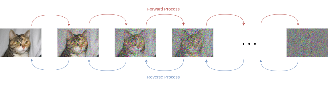

fw reverse process — Forward and reverse processes of diffustion models.

3. Diffusion Models structure

3.1. Diffusion Models as Hierarchical VAEs

DMs can be considered a form of hierarchical VAEs (H-VAEs): instead of one latent variable, multiple are learned \(\mathbf{z}_1, \mathbf{z}_2, \dots, \mathbf{z}_T\), which we refer to from now on using the notation \(\mathbf{z}_{1:T}\). In this context, each variable \(\mathbf{z}_t\) depends only on its predecessor \(\mathbf{z}_{t-1}\) such that \[ q_{\mathbf{z}_{1:T} | \mathbf{x}} (\mathbf{z}_{1:T} | \mathbf{x}_{i} ; \boldsymbol{\phi}_{1:T}) = q_{\mathbf{z}_{N} | \mathbf{x}} (\mathbf{z}_{N} | \mathbf{x}_{i} ; \boldsymbol{\phi}_{N}) \cdot \prod_{t=2}^{T} q_{\mathbf{z}_{t} | \mathbf{z}_{t-1}} (\mathbf{z}_{t} | \mathbf{z}_{t-1} ; \boldsymbol{\phi}_{t}) \] where \(q_{\mathbf{z}|\mathbf{x}}\) is the amortized variational posterior with parameters \(\boldsymbol{\phi}\).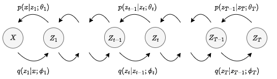

H-VAEs can be trained based on the MLE principle and following the variational approach similar to regular VAEs: VAEs: \[ \log p_{\mathbf{x}} (\mathbf{x} | \mathbf{z} ; \boldsymbol{\theta}, \boldsymbol{\phi}) \geq \mathrm{ELBO} = \mathbb{E}_{\mathbf{z} \sim q_{\mathbf{z}|\mathbf{x}}} \left[ \log \frac{p_{\mathbf{x}, \mathbf{z}} (\mathbf{x}, \mathbf{z} ; \boldsymbol{\theta})}{q_{\mathbf{z}|\mathbf{x}} (\mathbf{z} | \mathbf{x} ; \boldsymbol{\phi})} \right] \] H-VAEs: \[ \log p_{\mathbf{x}} (\mathbf{x} ; \boldsymbol{\theta}_{1:T}, \boldsymbol{\phi}_{1:T}) \geq \mathbb{E}_{\mathbf{z}_{1:T} \sim q_{\mathbf{z}_{1:T} | \mathbf{x}}} \left[ \log \frac{p_{\mathbf{x}, \mathbf{z}_{1:T}} (\mathbf{x}, \mathbf{z}_{1:T} ; \boldsymbol{\theta}_{1:T})}{q_{\mathbf{z}_{1:T} | \mathbf{x}} (\mathbf{z}_{1:T} | \mathbf{x} ; \boldsymbol{\phi}_{1:T})} \right] \] \[ \log p_{\mathbf{x}} (\mathbf{x} ; \boldsymbol{\theta}_{1:T}, \boldsymbol{\phi}_{1:T}) \geq \mathbb{E}_{\mathbf{z}_{1:T} \sim q_{\mathbf{z}_{1:T} | \mathbf{x}}} \left[ \log \frac{p_{\mathbf{z}_{1}} (\mathbf{z}_{1}) \ p_{\mathbf{x}} (\mathbf{x} | \mathbf{z}_{1:T} ; \boldsymbol{\theta}_{1:T}) \ \prod_{t=2}^{T} p_{\mathbf{z}_{t} | \mathbf{z}_{t-1}} (\mathbf{z}_{t} | \mathbf{z}_{t-1} ; \boldsymbol{\theta}_{t})}{q_{\mathbf{z}_{N}|\mathbf{x}} (\mathbf{z}_{N} | \mathbf{x} ; \boldsymbol{\phi}_{N}) \cdot \prod_{t=2}^{T} q_{\mathbf{z}_{t} | \mathbf{z}_{t-1}} (\mathbf{z}_{t} | \mathbf{z}_{t-1} ; \boldsymbol{\phi}_{t})} \right] \] However, optimizing the parameters \(\boldsymbol{\theta}\) and \(\boldsymbol{\phi}\) using this expression results in highly complex training. In this post, we focus on the vanilla DM architecture, which is slightly different:

\(\mathbf{X}_t := \mathbf{Z}_t\) and all \(\mathbf{X}_t\) with \(t \in \{1, \dots, T\}\) have the same dimension \(D\) as the data, where \(\mathbf{X}_0\) denotes a datasample.
The Encoder is fixed and used iteratively in the forward process, which is by design a Markov process.
Only the reverse process is learned.

3.2. Forward Process

3.2.1. Noise Schedule

For each timestep \(t\), we sample \(\boldsymbol{\epsilon} \sim \mathcal{N}(\mathbf{0}, \mathbf{I})\) and add it to samples \(\mathbf{x}_t\) iteratively as follows: \[ \mathbf{x}_{t} = \sqrt{\alpha_{t}} \mathbf{x}_{t-1} + \sqrt{1 – \alpha_{t}} \boldsymbol{\epsilon}_{t-1}, \quad \alpha_{t} \in (0, 1) \] where \(\alpha_t\) is a hyperparameter that determines the noise schedule, thus controlling the smoothness of the diffusion process. This choice of coefficients ensures that the mean of \(\mathbf{x}_t\) is closer to zero than the mean of \(\mathbf{x}_{t-1}\) and the variance of \(\mathbf{x}_t\) is closer to the unit matrix than the variance of \(\mathbf{x}_{t-1}\). The transformation can be written in the form: \[ q_{\mathbf{x}_{t} | \mathbf{x}_{t-1}} (\mathbf{x}_{t} | \mathbf{x}_{t-1}) = \mathcal{N} \left( \mathbf{x}_{t} ; \sqrt{\alpha_{t}} \mathbf{x}_{t-1}, (1 – \alpha_{t}) \mathbf{I} \right) \] There are different options for the noise schedule. Usually, we define a function that determines \(\alpha_t\) at each timestep \(t\). Common noise schedules in literature are linear, geometric, and cosine. For example: \[ \alpha_{t} = 1 – \left[ (\max – \min) \frac{t}{T} + \min \right] \] \[ \text{where } \max, \min \in [0, 1] \text{ are two small constants, } \min < \max, \] \[ \text{and } T \text{ is the total number of timesteps.} \] The given function will compute a sequence of \(\alpha_1, \dots, \alpha_T\) that interpolate linearly between \(\min\) and \(\max\). While the original paper uses \(\alpha\) to denote the noise schedule, another notation used in the literature is \(\beta_t := 1-\alpha_t\). The corresponding equation is then: \[ \mathbf{x}_{t} = \sqrt{1 – \beta_{t}} \mathbf{x}_{t-1} + \sqrt{\beta_{t}} \boldsymbol{\epsilon}_{t-1} \] To further understand the role of \(\alpha\), we can refer to the visualization below . The figure shows how \(\alpha\) controls the transition from a sample \(\mathbf{x}_t\) to a noisier sample \(\mathbf{x}_{t+1}\), which in turn controls the complexity of learning for the model and thus the quality of sampling. A trade-off is needed to balance sampling quality and training feasibility (by keeping the number of timesteps relatively short).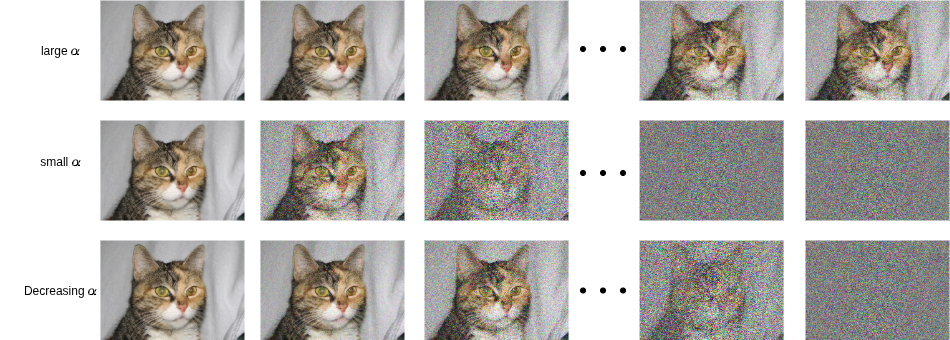

3.2.2. Diffusion Kernel

The diffusion kernel is the function that defines the transformation in the forward process, which is the same as the PDF of a Gaussian distribution. It can be derived as follows: \[ \mathbf{x}_{t} = \sqrt{\alpha_{t}} \mathbf{x}_{t-1} + \sqrt{1 – \alpha_{t}} \boldsymbol{\epsilon}_{t-1}, \quad \boldsymbol{\epsilon}_{t-1} \sim \mathcal{N}(\mathbf{0}, \mathbf{I}) \] \[ = \sqrt{\alpha_{t}} \left( \sqrt{\alpha_{t-1}} \mathbf{x}_{t-2} + \sqrt{1 – \alpha_{t-1}} \boldsymbol{\epsilon}_{t-2} \right) + \sqrt{1 – \alpha_{t}} \boldsymbol{\epsilon}_{t-1} \] \[ = \sqrt{\alpha_{t} \alpha_{t-1}} \mathbf{x}_{t-2} + \sqrt{\alpha_{t} (1 – \alpha_{t-1})} \boldsymbol{\epsilon}_{t-2} + \sqrt{1 – \alpha_{t}} \boldsymbol{\epsilon}_{t-1} \] \[ \stackrel{(*)}{=} \sqrt{\alpha_{t} \alpha_{t-1}} \mathbf{x}_{t-2} + \sqrt{\alpha_{t} (1 – \alpha_{t-1}) + (1 – \alpha_{t})} \boldsymbol{\epsilon}_{t-2}^{*} \] \[ \cdots \] \[ = \sqrt{\prod_{\tau=1}^{t} \alpha_{\tau}} \mathbf{x}_{0} + \sqrt{1 – \prod_{\tau=1}^{t} \alpha_{\tau}} \boldsymbol{\epsilon}_{0} \] \[ = \sqrt{\bar{\alpha}_{t}} \mathbf{x}_{0} + \sqrt{1 – \bar{\alpha}_{t}} \boldsymbol{\epsilon}_{0}, \quad \boldsymbol{\epsilon}_{0} \sim \mathcal{N}(\mathbf{0}, \mathbf{I}), \quad \bar{\alpha}_{t} = \prod_{\tau=1}^{t} \alpha_{\tau} \] \[ \text{(*) Sum of 2 independent Gaussians is again Gaussian.} \] This leads to the forward Gaussian Kernel: \[ q_{\mathbf{x}_{t} | \mathbf{x}_{0}} (\mathbf{x}_{t} | \mathbf{x}_{0}) = \mathcal{N} \left( \mathbf{x}_{t} ; \sqrt{\bar{\alpha}_{t}} \mathbf{x}_{0}, (1 – \bar{\alpha}_{t}) \mathbf{I} \right) \]

The **Gaussian Diffusion kernel** preserves the norm of \(\mathbf{x}\) across the **diffusion process**, which is beneficial for training stability. The following derivation proves it:\[ \mathbb{E}_{\mathbf{x}_{t} | \mathbf{x}_{0}} [\|\mathbf{x}_{t}\|_{2}^{2}] = \mathbb{E}_{\mathbf{x}_{0}, \boldsymbol{\epsilon}} \left[ \left\| \sqrt{\bar{\alpha}_{t}} \mathbf{x}_{0} + \sqrt{1 – \bar{\alpha}_{t}} \boldsymbol{\epsilon} \right\|^{2} \right] \] \[ = \mathbb{E}_{\mathbf{x}_{0}, \boldsymbol{\epsilon}} \left[ \left( \sqrt{\bar{\alpha}_{t}} \mathbf{x}_{0} + \sqrt{1 – \bar{\alpha}_{t}} \boldsymbol{\epsilon} \right)^{\top} \left( \sqrt{\bar{\alpha}_{t}} \mathbf{x}_{0} + \sqrt{1 – \bar{\alpha}_{t}} \boldsymbol{\epsilon} \right) \right] \] \[ = \mathbb{E}_{\mathbf{x}_{0}, \boldsymbol{\epsilon}} \left[ \bar{\alpha}_{t} \mathbf{x}_{0}^{\top} \mathbf{x}_{0} + 2 \sqrt{\bar{\alpha}_{t} (1 – \bar{\alpha}_{t})} \boldsymbol{\epsilon}^{\top} \mathbf{x}_{0} + (1 – \bar{\alpha}_{t}) \boldsymbol{\epsilon}^{\top} \boldsymbol{\epsilon} \right] \] \[ = \bar{\alpha}_{t} \mathbb{E}_{\mathbf{x}_{0}} [\|\mathbf{x}_{0}\|^{2}] + (1 – \bar{\alpha}_{t}) \mathbb{E}_{\boldsymbol{\epsilon}} [\|\boldsymbol{\epsilon}\|^{2}] \] \[ = \bar{\alpha}_{t} D + (1 – \bar{\alpha}_{t}) D = D, \quad D \text{ is the dimension of } \mathbf{x}_{0} \]Before moving to the reverse process, let us summarize the forward process. As already mentioned, the forward process is not parametrized; \(\alpha_t\) is a hyperparameter that controls the generation quality and impacts the **training complexity**. Based on the chain rule of probability, the joint distribution of the latent representations \(\mathbf{x}_t\) where \(t = 1, 2, \dots, T\), conditioned on the observed data \(\mathbf{x}_0\), is given by

\[ q (\mathbf{x}_{1}, \ldots, \mathbf{x}_{T} | \mathbf{x}_{0}) = q(\mathbf{x}_{1} | \mathbf{x}_{0}) \cdot q(\mathbf{x}_{2} | \mathbf{x}_{1}, \mathbf{x}_{0}) \cdots q(\mathbf{x}_{T} | \mathbf{x}_{T-1}, \ldots, \mathbf{x}_{0}) \] The fact that the forward process is non-parametrized (the encoder is fixed and not learned as in VAEs) makes it a Markov chain; that is, each **noising step** depends only on the previous step. This simplifies the expression: \[ q (\mathbf{x}_{1}, \ldots, \mathbf{x}_{T} | \mathbf{x}_{0}) = q(\mathbf{x}_{1} | \mathbf{x}_{0}) \cdot q(\mathbf{x}_{2} | \mathbf{x}_{1}) \cdots q(\mathbf{x}_{T} | \mathbf{x}_{T-1}) \] with the more compact notation: \[ q (\mathbf{x}_{1:T} | \mathbf{x}_{0}) = \prod_{t=1}^{T} q(\mathbf{x}_{t} | \mathbf{x}_{t-1}) \] The Diffusion kernel, which is equivalent to a Gaussian kernel, allows us to transform the observed sample \(\mathbf{x}_0\) to an arbitrary representation \(\mathbf{x}_t\), again following the expression: \[ q_{\mathbf{x}_{t} | \mathbf{x}_{0}} (\mathbf{x}_{t} | \mathbf{x}_{0}) = \mathcal{N} \left( \mathbf{x}_{t} ; \sqrt{\bar{\alpha}_{t}} \mathbf{x}_{0}, (1 – \bar{\alpha}_{t}) \mathbf{I} \right) \]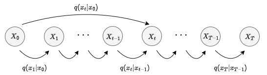

3.3. Reverse Process

The Reverse process is the process of reversing the diffusion or simply denoising. To achieve this, we need the transformation from \(\mathbf{x}_t\) to \(\mathbf{x}_{t-1}\). More precisely, we need the posterior distribution \(q(\mathbf{x}_{t-1}|\mathbf{x}_t)\). The common method to obtain the posterior is Bayesian inference: \[ q(\mathbf{x}_{t-1} | \mathbf{x}_{t}) = \frac{q(\mathbf{x}_{t} | \mathbf{x}_{t-1}) q(\mathbf{x}_{t-1})}{q(\mathbf{x}_{t})} \] However, similar to the models we learned so far, the posterior is intractable to compute again because of \(q(\mathbf{x}_t)\) in the denominator. More precisely, this is due to the expression of \(q(\mathbf{x}_t)\) that depends on \(q(\mathbf{x}_0)\) through marginalization. \(q(\mathbf{x}_0)\) is the likelihood or data distribution that we do not know and intend to model with the DM, as the following expression demonstrates: \[ q(\mathbf{x}_{t}) = \int_{\mathbf{x}_{t-1}, \ldots, \mathbf{x}_{0}} q(\mathbf{x}_{t:0}) \, d\mathbf{x}_{t-1} \cdots d\mathbf{x}_{0} \] \[ = \int_{\mathbf{x}_{t-1}, \ldots, \mathbf{x}_{0}} q(\mathbf{x}_{0}) \prod_{\tau=1}^{t} q(\mathbf{x}_{\tau} | \mathbf{x}_{\tau-1}) \, d\mathbf{x}_{t-1} \cdots d\mathbf{x}_{0} \] We conclude that we end up in the same setup as VAE. To get around this problem, we approximate the reverse distribution \(q(\mathbf{x}_{t-1}|\mathbf{x}_t)\) with a distribution \(p(\mathbf{x}_{t-1}|\mathbf{x}_t;\boldsymbol{\theta})\), similar to the variational inference strategy in VAEs. To avoid confusion, recall that in VAE the notation is reversed; that is, the posterior PDF \(p(\mathbf{z}|\mathbf{x})\) is approximated with the variational posterior \(q(\mathbf{z}|\mathbf{x};\boldsymbol{\phi})\). The approximate distribution \(p(\mathbf{x}_{t-1}|\mathbf{x}_t;\boldsymbol{\theta})\) is learned with a deep neural network with parameters \(\boldsymbol{\theta}\). In vanilla DMs, this approximate posterior is defined as a normal distribution, which means the deep neural network is a density net (learns a data distribution) with input \(\mathbf{x}_t\) and \(t\), parameters \(\boldsymbol{\theta}\), and output the mean \(\boldsymbol{\mu}_{\boldsymbol{\theta}}(\mathbf{x}_{t}, t)\) and covariance matrix \(\mathbf{C}_{\boldsymbol{\theta}}(\mathbf{x}_{t}, t)\): \[ p(\mathbf{x}_{t-1} | \mathbf{x}_{t} ; \boldsymbol{\theta}) = \mathcal{N} \left( \mathbf{x}_{t-1} ; \boldsymbol{\mu}_{\boldsymbol{\theta}}(\mathbf{x}_{t}, t), \mathbf{C}_{\boldsymbol{\theta}}(\mathbf{x}_{t}, t) \right) \] To reduce complexity, instead of learning \(T\) different networks with parameters \(\boldsymbol{\theta}_1, \dots, \boldsymbol{\theta}_T\), we learn a single network and use it for all steps, given that we provide the step index \(t\) as input. This principle is called parameter sharing. Moreover, the authors simplify the model further by keeping the variance constant instead of learning \(\mathbf{C}_{\boldsymbol{\theta}}(\mathbf{x}_{t}, t)\) explicitly. The final reverse model is: \[ p(\mathbf{x}_{t-1} | \mathbf{x}_{t} ; \boldsymbol{\theta}) = \mathcal{N} \left( \mathbf{x}_{t-1} ; \boldsymbol{\mu}_{\boldsymbol{\theta}}(\mathbf{x}_{t}, t), \sigma_{t}^{2} \mathbf{I} \right) \] The paper mentions that setting \(\sigma_t = 1 – \alpha_t = \beta_t\) works well in practice. The complete reverse process can be formulated as: \[ p_{\boldsymbol{\theta}} (\mathbf{x}_{0:T}) = p(\mathbf{x}_{T} ; \boldsymbol{\theta}) \prod_{t=1}^{T} p(\mathbf{x}_{t-1} | \mathbf{x}_{t} ; \boldsymbol{\theta}) \] Notice that \(p(\mathbf{x}_{0:T};\boldsymbol{\theta})\) is unconditioned, unlike \(q(\mathbf{x}_{1:T}|\mathbf{x}_0)\) from the forward process, which needs \(\mathbf{x}_0\) as input. In the reverse process, we just start from Gaussian noise.

4. Diffusion Models Training

4.1. ELBO

The obvious approach to train probabilistic generative modeling is to use the log likelihood function as an objective and optimize the parameters of the model to maximize it, or in practice, to minimize its negative. As already mentioned, the likelihood function is intractable, so we maximize a lower bound on the likelihood, which is the Evidence Lower Bound (ELBO) similar to that used with variational autoencoders. We start by deriving the ELBO for diffusion models, which is very similar to the ELBO for VAEs, except that there are now multiple encoder and decoder stages: \[ \log p_{\mathbf{x}} (\mathbf{x}_{0} ; \boldsymbol{\theta}) = \mathrm{ELBO} + D_{\mathrm{KL}} \left( q(\mathbf{x}_{1:T} | \mathbf{x}_{0}) \| p_{\boldsymbol{\theta}}(\mathbf{x}_{1:T} | \mathbf{x}_{0}) \right) \] \[ \mathrm{ELBO} = \mathbb{E}_{\mathbf{x}_{1:T} \sim q_{\mathbf{x}_{1:T} | \mathbf{x}_{0}}} \left[ \log \frac{p(\mathbf{x}_{T}) \cdot \prod_{t=1}^{T} p(\mathbf{x}_{t-1} | \mathbf{x}_{t} ; \boldsymbol{\theta})}{\prod_{t=1}^{T} q(\mathbf{x}_{t} | \mathbf{x}_{t-1})} \right] \] \[ = \mathbb{E}_{\mathbf{x}_{1:T} \sim q_{\mathbf{x}_{1:T} | \mathbf{x}_{0}}} \left[ \log \frac{p(\mathbf{x}_{T}) P(\mathbf{x}_{0} | \mathbf{x}_{1} ; \boldsymbol{\theta})}{q(\mathbf{x}_{1} | \mathbf{x}_{0})} + \log \prod_{t=2}^{T} \frac{P(\mathbf{x}_{t-1} | \mathbf{x}_{t} ; \boldsymbol{\theta})}{q(\mathbf{x}_{t} | \mathbf{x}_{t-1})} \right] \] \[ = \mathbb{E}_{\mathbf{x}_{1:T} \sim q_{\mathbf{x}_{1:T} | \mathbf{x}_{0}}} \left[ \log \frac{p(\mathbf{x}_{T}) P(\mathbf{x}_{0} | \mathbf{x}_{1} ; \boldsymbol{\theta})}{q(\mathbf{x}_{1} | \mathbf{x}_{0})} + \mathbb{A} \right] \] The last step is done to separate the terms that map between \(\mathbf{x}_0\) and \(\mathbf{x}_1\) (we will see why later) and also because we want to write the ELBO in terms of Kullback-Leibler divergences to find a closed-form expression. Next, we use Bayesian inference to simplify \(\mathbb{A}\): \[ q(\mathbf{x}_{t-1} | \mathbf{x}_{t}, \mathbf{x}_{0}) = \frac{q(\mathbf{x}_{t} | \mathbf{x}_{t-1}, \mathbf{x}_{0}) q(\mathbf{x}_{t-1} | \mathbf{x}_{0})}{q(\mathbf{x}_{t} | \mathbf{x}_{0})} \quad \text{(Bayesian inference)} \] \[ \mathbb{A} = \log \prod_{t=2}^{T} \frac{q(\mathbf{x}_{t-1} | \mathbf{x}_{0}) \cdot p(\mathbf{x}_{t-1} | \mathbf{x}_{t} ; \boldsymbol{\theta})}{q(\mathbf{x}_{t} | \mathbf{x}_{0})} \] \[ = \log \frac{q(\mathbf{x}_{T-1} | \mathbf{x}_{0}) \cdots q(\mathbf{x}_{1} | \mathbf{x}_{0})}{q(\mathbf{x}_{T} | \mathbf{x}_{0}) \cdots q(\mathbf{x}_{2} | \mathbf{x}_{0})} + \log \prod_{t=2}^{T} \frac{p(\mathbf{x}_{t-1} | \mathbf{x}_{t} ; \boldsymbol{\theta})}{q(\mathbf{x}_{t} | \mathbf{x}_{t-1}, \mathbf{x}_{0})} \] \[ = \log \frac{q(\mathbf{x}_{1} | \mathbf{x}_{0})}{q(\mathbf{x}_{T} | \mathbf{x}_{0})} + \log \prod_{t=2}^{T} \frac{p(\mathbf{x}_{t-1} | \mathbf{x}_{t} ; \boldsymbol{\theta})}{q(\mathbf{x}_{t-1} | \mathbf{x}_{t}, \mathbf{x}_{0})} \] Now we go back to the **ELBO** expression: \[ = \mathbb{E}_{\mathbf{x}_{1:T} \sim q_{\mathbf{x}_{1:T} | \mathbf{x}_{0}}} \left[ \log \frac{P(\mathbf{x}_{T}) P(\mathbf{x}_{0} | \mathbf{x}_{1} ; \boldsymbol{\theta})}{q(\mathbf{x}_{1} | \mathbf{x}_{0})} + \log \frac{q(\mathbf{x}_{1} | \mathbf{x}_{0})}{q(\mathbf{x}_{T} | \mathbf{x}_{0})} + \log \prod_{t=2}^{T} \frac{P(\mathbf{x}_{t-1} | \mathbf{x}_{t} ; \boldsymbol{\theta})}{q(\mathbf{x}_{t-1} | \mathbf{x}_{t}, \mathbf{x}_{0})} \right] \] \[ = \mathbb{E}_{\mathbf{x}_{1:T} \sim q_{\mathbf{x}_{1:T} | \mathbf{x}_{0}}} \left[ \log \frac{P(\mathbf{x}_{T}) P(\mathbf{x}_{0} | \mathbf{x}_{1} ; \boldsymbol{\theta})}{q(\mathbf{x}_{T} | \mathbf{x}_{0})} + \sum_{t=2}^{T} \log \frac{P(\mathbf{x}_{t-1} | \mathbf{x}_{t} ; \boldsymbol{\theta})}{q(\mathbf{x}_{t-1} | \mathbf{x}_{t}, \mathbf{x}_{0})} \right] \] \[ = \mathbb{E}_{\mathbf{x}_{1:T} \sim q_{\mathbf{x}_{1:T} | \mathbf{x}_{0}}} \left[ \log P(\mathbf{x}_{0} | \mathbf{x}_{1} ; \boldsymbol{\theta}) + \log \frac{P(\mathbf{x}_{T})}{q(\mathbf{x}_{T} | \mathbf{x}_{0})} + \sum_{t=2}^{T} \log \frac{P(\mathbf{x}_{t-1} | \mathbf{x}_{t} ; \boldsymbol{\theta})}{q(\mathbf{x}_{t-1} | \mathbf{x}_{t}, \mathbf{x}_{0})} \right] \] \[ \implies \mathrm{ELBO} = \mathbb{E}_{\mathbf{x}_{1} \sim q_{\mathbf{x}_{1} | \mathbf{x}_{0}}} \left[ \log P(\mathbf{x}_{0} | \mathbf{x}_{1} ; \boldsymbol{\theta}) \right] + \mathbb{E}_{\mathbf{x}_{T} \sim q_{\mathbf{x}_{T} | \mathbf{x}_{0}}} \left[ \log \frac{P(\mathbf{x}_{T})}{q(\mathbf{x}_{T} | \mathbf{x}_{0})} \right] \] \[ + \sum_{t=2}^{T} \mathbb{E}_{\mathbf{x}_{t-1}, \mathbf{x}_{t} \sim q_{\mathbf{x}_{t-1}, \mathbf{x}_{t} | \mathbf{x}_{0}}} \left[ \log \frac{P(\mathbf{x}_{t-1} | \mathbf{x}_{t} ; \boldsymbol{\theta})}{q(\mathbf{x}_{t-1} | \mathbf{x}_{t}, \mathbf{x}_{0})} \right] \] \[ = \alpha + \beta + \gamma \] Next, we use \(D_{\mathrm{KL}} (q\|p) = \mathbb{E}_q[\log \frac{q}{p}]\) to analyze the terms: \[ \alpha = \mathbb{E}_{\mathbf{x}_{1} \sim q_{\mathbf{x}_{1} | \mathbf{x}_{0}}} [\log P(\mathbf{x}_{0} | \mathbf{x}_{1} ; \boldsymbol{\theta})] \] \[ \beta = \mathbb{E}_{\mathbf{x}_{T} \sim q_{\mathbf{x}_{T} | \mathbf{x}_{0}}} \left[ \log \frac{P(\mathbf{x}_{T})}{q(\mathbf{x}_{T} | \mathbf{x}_{0})} \right] = – D_{\mathrm{KL}} \left( q(\mathbf{x}_{T} | \mathbf{x}_{0}) \| P(\mathbf{x}_{T}) \right) \] \[ \gamma = \sum_{t=2}^{T} \mathbb{E}_{\mathbf{x}_{t}, \mathbf{x}_{t-1} \sim q_{\mathbf{x}_{t}, \mathbf{x}_{t-1} | \mathbf{x}_{0}}} \left[ \log \frac{P(\mathbf{x}_{t-1} | \mathbf{x}_{t} ; \boldsymbol{\theta})}{q(\mathbf{x}_{t-1} | \mathbf{x}_{t}, \mathbf{x}_{0})} \right] \] The terms \(\alpha\), \(\beta\), \(\gamma\) have specific meanings in the literature:

\(\alpha\): This is called the reconstruction term because it is higher if the model successfully reconstructs the sample \(\mathbf{x}_0\) from the noisy representation \(\mathbf{x}_1\). This term may be ignored in training because it is very small and the model has already recovered most of the sample.
\(\beta\): The prior matching term can be ignored as well because it does not depend on \(\boldsymbol{\theta}\).
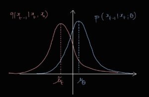
\(\gamma\): The consistency term or denoising matching term measures how well the model performs reverse diffusion. It is a measure of how close the trainable transition \(p_{\mathbf{x}_{t-1}|\mathbf{x}_t}\) is to the true posterior \(q_{\mathbf{x}_{t-1}|\mathbf{x}_t,\mathbf{x}_0}\), which is semi-aided by the knowledge of \(\mathbf{x}_0\).

For training, we need to further simplify \(\gamma\): \[ \gamma = \sum_{t=2}^{T} \mathbb{E}_{\mathbf{x}_{t}, \mathbf{x}_{t-1} \sim q_{\mathbf{x}_{t}, \mathbf{x}_{t-1} | \mathbf{x}_{0}}} \left[ \log \frac{P(\mathbf{x}_{t-1} | \mathbf{x}_{t} ; \boldsymbol{\theta})}{q(\mathbf{x}_{t-1} | \mathbf{x}_{t}, \mathbf{x}_{0})} \right] \] \[ \stackrel{(*)}{=} \sum_{t=2}^{T} \mathbb{E}_{\mathbf{x}_{t} \sim q_{\mathbf{x}_{t} | \mathbf{x}_{0}}} \left[ \mathbb{E}_{\mathbf{x}_{t-1} \sim q_{\mathbf{x}_{t-1} | \mathbf{x}_{t}, \mathbf{x}_{0}}} \left[ \log \frac{P(\mathbf{x}_{t-1} | \mathbf{x}_{t} ; \boldsymbol{\theta})}{q(\mathbf{x}_{t-1} | \mathbf{x}_{t}, \mathbf{x}_{0})} \right] \right] \] \[ = – \sum_{t=2}^{T} \mathbb{E}_{\mathbf{x}_{t} \sim q_{\mathbf{x}_{t} | \mathbf{x}_{0}}} \left[ D_{\mathrm{KL}} \left( q(\mathbf{x}_{t-1} | \mathbf{x}_{t}, \mathbf{x}_{0}) \| P_{\boldsymbol{\theta}}(\mathbf{x}_{t-1} | \mathbf{x}_{t}) \right) \right] \] \[ \text{(*) Here we used the law of total expectation } \mathbb{E}_{\mathbf{x}, \mathbf{y}} [g(\mathbf{x}, \mathbf{y})] = \mathbb{E}_{\mathbf{y}} [\mathbb{E}_{\mathbf{x} | \mathbf{y}} [g(\mathbf{x}, \mathbf{y})]] \] \[ \text{and the product rule: } q_{\mathbf{x}_{t}, \mathbf{x}_{t-1} | \mathbf{x}_{0}} = q_{\mathbf{x}_{t-1} | \mathbf{x}_{t}, \mathbf{x}_{0}} \cdot q_{\mathbf{x}_{t} | \mathbf{x}_{0}} \] Now we derive the analytic expression of each **PDF** separately, starting with \(q(\mathbf{x}_{t-1} | \mathbf{x}_{t}, \mathbf{x}_{0})\): \[ q(\mathbf{x}_{t-1} | \mathbf{x}_{t}, \mathbf{x}_{0}) = \frac{q(\mathbf{x}_{t} | \mathbf{x}_{t-1}, \mathbf{x}_{0}) \cdot q(\mathbf{x}_{t-1} | \mathbf{x}_{0})}{q(\mathbf{x}_{t} | \mathbf{x}_{0})} \quad \text{(product rule again)} \] \[ = \frac{q(\mathbf{x}_{t} | \mathbf{x}_{t-1}) \cdot q(\mathbf{x}_{t-1} | \mathbf{x}_{0})}{q(\mathbf{x}_{t} | \mathbf{x}_{0})} \quad \text{(Markov chain)} \] \[ = \frac{\mathcal{N} (\mathbf{x}_{t} ; \sqrt{\alpha_{t}} \mathbf{x}_{t-1}, (1 – \alpha_{t}) \mathbf{I}) \cdot \mathcal{N} (\mathbf{x}_{t-1} ; \sqrt{\bar{\alpha}_{t-1}} \mathbf{x}_{0}, (1 – \bar{\alpha}_{t-1}) \mathbf{I})}{\mathcal{N} (\mathbf{x}_{t} ; \sqrt{\bar{\alpha}_{t}} \mathbf{x}_{0}, (1 – \bar{\alpha}_{t}) \mathbf{I})} \] \[ = \frac{\exp \left( \frac{-1}{2(1-\alpha_{t})} \| \mathbf{x}_{t} – \sqrt{\alpha_{t}} \mathbf{x}_{t-1} \|^{2} \right) \cdot \exp \left( \frac{-1}{2(1-\bar{\alpha}_{t-1})} \| \mathbf{x}_{t-1} – \sqrt{\bar{\alpha}_{t-1}} \mathbf{x}_{0} \|^{2} \right)}{\exp \left( \frac{-1}{2(1-\bar{\alpha}_{t})} \| \mathbf{x}_{t} – \sqrt{\bar{\alpha}_{t}} \mathbf{x}_{0} \|^{2} \right)} \] Then, using the rules of the product of two **Gaussians** \(\mathcal{N}(\mathbf{x}_{t-1} ; \boldsymbol{\mu}_{1}, \mathbf{\Sigma}_{1})\) and \(\mathcal{N}(\mathbf{x}_{t-1} ; \boldsymbol{\mu}_{2}, \mathbf{\Sigma}_{2})\): \[ \mathbf{C} = (\mathbf{\Sigma}_{1}^{-1} + \mathbf{\Sigma}_{2}^{-1})^{-1}, \quad \boldsymbol{\mu} = \mathbf{C} (\mathbf{\Sigma}_{1}^{-1} \boldsymbol{\mu}_{1} + \mathbf{\Sigma}_{2}^{-1} \boldsymbol{\mu}_{2}) \] we obtain: \[ q(\mathbf{x}_{t-1} | \mathbf{x}_{t}, \mathbf{x}_{0}) = \mathcal{N} \left( \mathbf{x}_{t-1} ; \boldsymbol{\mu}_{\mathbf{x}_{t-1} | \mathbf{x}_{t}, \mathbf{x}_{0}}, \sigma^{2}_{\mathbf{x}_{t-1} | \mathbf{x}_{t}, \mathbf{x}_{0}} \mathbf{I} \right) \] \[ \text{with:} \] \[ \boldsymbol{\mu}_{\mathbf{x}_{t-1} | \mathbf{x}_{t}, \mathbf{x}_{0}} = \frac{\sqrt{\alpha_{t}} (1 – \bar{\alpha}_{t-1})}{1 – \bar{\alpha}_{t}} \mathbf{x}_{t} + \frac{\sqrt{\bar{\alpha}_{t-1}} (1 – \alpha_{t})}{1 – \bar{\alpha}_{t}} \mathbf{x}_{0} = \frac{\sqrt{\alpha_{t}} (1 – \bar{\alpha}_{t-1})}{1 – \bar{\alpha}_{t}} \mathbf{x}_{t} + \frac{\sqrt{\bar{\alpha}_{t-1}} \beta_{t}}{1 – \bar{\alpha}_{t}} \mathbf{x}_{0} \] \[ \sigma^{2}_{\mathbf{x}_{t-1} | \mathbf{x}_{t}, \mathbf{x}_{0}} = \frac{(1-\alpha_{t})(1-\bar{\alpha}_{t-1})}{1-\bar{\alpha}_{t}} = \frac{1-\alpha_{t}}{1-\bar{\alpha}_{t}} (1-\bar{\alpha}_{t-1}) = \tilde{\beta}_{t} \] We repeat the same steps for \(P_{\boldsymbol{\theta}}(\mathbf{x}_{t-1} | \mathbf{x}_{t})\) to get: \[ p_{\mathbf{x}_{t-1} | \mathbf{x}_{t}} (\mathbf{x}_{t-1} | \mathbf{x}_{t} ; \boldsymbol{\theta}) = \mathcal{N} \left( \mathbf{x}_{t-1} ; \boldsymbol{\mu}_{\mathbf{x}_{t-1} | \mathbf{x}_{t}} (\mathbf{x}_{t} ; \boldsymbol{\theta}), \mathbf{C}_{\mathbf{x}_{t-1} | \mathbf{x}_{t}} (\mathbf{x}_{t} ; \boldsymbol{\theta}) \right) \] As already mentioned in the previous section, the covariance matrices are fixed (not learned): \[ \mathbf{C}_{\mathbf{x}_{t-1} | \mathbf{x}_{t}} (\mathbf{x}_{t} ; \boldsymbol{\theta}) = \sigma^{2}_{\mathbf{x}_{t-1} | \mathbf{x}_{t}} \mathbf{I} = \tilde{\beta}_{t} \mathbf{I} \] This simplifies the model but also matches the covariances of the true but not accessible posterior \(q_{\mathbf{x}_{t-1}|\mathbf{x}_t,\mathbf{x}_0}\). To simplify notation, we use the following for the rest of the derivation: \[ \tilde{\boldsymbol{\mu}}_{t} := \boldsymbol{\mu}_{\mathbf{x}_{t-1} | \mathbf{x}_{t}, \mathbf{x}_{0}}, \quad \text{mean of non-accessible true posterior} \] \[ \boldsymbol{\mu}_{\boldsymbol{\theta}} := \boldsymbol{\mu}_{\mathbf{x}_{t-1} | \mathbf{x}_{t}}, \quad \text{mean of the approximate posterior obtained with means of NNs} \] \[ \tilde{\sigma}^{2}_{t} := \sigma^{2}_{\mathbf{x}_{t-1} | \mathbf{x}_{t}}, \quad \text{variance of both posteriors} \] Next, we use the obtained expressions and the rule of Kullback-Leibler divergence for two **Gaussians** \(P \sim \mathcal{N}(\boldsymbol{\mu}_1, \mathbf{C}_1)\) and \(Q \sim \mathcal{N}(\boldsymbol{\mu}_2, \mathbf{C}_2)\) with vector space dimensionality \(D\): \[ D_{\mathrm{KL}} (P \| Q) = \frac{1}{2} \left[ (\boldsymbol{\mu}_{2} – \boldsymbol{\mu}_{1})^{\top} \mathbf{C}_{2}^{-1} (\boldsymbol{\mu}_{2} – \boldsymbol{\mu}_{1}) + \mathrm{tr}(\mathbf{C}_{2}^{-1} \mathbf{C}_{1}) + \log \left( \frac{\det(\mathbf{C}_{2})}{\det(\mathbf{C}_{1})} \right) – D \right] \] to get: \[ D_{\mathrm{KL}} \left( q(\mathbf{x}_{t-1} | \mathbf{x}_{t}, \mathbf{x}_{0}) \| p_{\boldsymbol{\theta}}(\mathbf{x}_{t-1} | \mathbf{x}_{t}) \right) \] \[ = \frac{1}{2} \left[ (\boldsymbol{\mu}_{\boldsymbol{\theta}} – \tilde{\boldsymbol{\mu}}_{t})^{\top} (\sigma_{t}^{2} \mathbf{I})^{-1} (\boldsymbol{\mu}_{\boldsymbol{\theta}} – \tilde{\boldsymbol{\mu}}_{t}) + \mathrm{tr}((\sigma_{t}^{2} \mathbf{I})^{-1} (\tilde{\sigma}_{t}^{2} \mathbf{I})) + \log \left( \frac{\det(\sigma_{t}^{2} \mathbf{I})}{\det(\tilde{\sigma}_{t}^{2} \mathbf{I})} \right) – D \right] \] \[ = \frac{1}{2} \left[ \frac{1}{\sigma_{t}^{2}} \| \boldsymbol{\mu}_{\boldsymbol{\theta}} – \tilde{\boldsymbol{\mu}}_{t} \|^{2} + D \cdot \frac{\tilde{\sigma}_{t}^{2}}{\sigma_{t}^{2}} + D \cdot \log \left( \frac{\sigma_{t}^{2}}{\tilde{\sigma}_{t}^{2}} \right) – D \right] \] \[ \text{Assuming } \sigma_{t}^{2} = \tilde{\sigma}_{t}^{2}: \] \[ = \frac{1}{2} \left[ \frac{1}{\sigma_{t}^{2}} \| \boldsymbol{\mu}_{\boldsymbol{\theta}} – \tilde{\boldsymbol{\mu}}_{t} \|^{2} + D + 0 – D \right] \] \[ = \frac{1}{2 \sigma_{t}^{2}} \| \boldsymbol{\mu}_{\boldsymbol{\theta}} – \tilde{\boldsymbol{\mu}}_{t} \|^{2} \] Finally, the obtained ELBO: \[ \mathrm{ELBO} \approx \gamma = – \sum_{t=2}^{T} \mathbb{E}_{\mathbf{x}_{t} \sim q_{\mathbf{x}_{t} | \mathbf{x}_{0}}} \left[ D_{\mathrm{KL}} \left( q(\mathbf{x}_{t-1} | \mathbf{x}_{t}, \mathbf{x}_{0}) \| p_{\boldsymbol{\theta}}(\mathbf{x}_{t-1} | \mathbf{x}_{t}) \right) \right] \] \[ = – \sum_{t=2}^{T} \mathbb{E}_{\mathbf{x}_{t} \sim q_{\mathbf{x}_{t} | \mathbf{x}_{0}}} \left[ \frac{1}{2 \sigma_{t}^{2}} \| \boldsymbol{\mu}_{\boldsymbol{\theta}} – \tilde{\boldsymbol{\mu}}_{t} \|^{2} \right] \] and the final Objective to optimize the parameters \(\boldsymbol{\theta}\) is equivalent to a Minimum Square Error (MSE) loss: \[ \hat{\boldsymbol{\theta}} = \underset{\boldsymbol{\theta}}{\arg \max} \sum_{i=1}^{N} \sum_{t=2}^{T} – \mathbb{E}_{\mathbf{x}_{t} \sim q_{\mathbf{x}_{t} | \mathbf{x}_{0}}} \left[ \frac{1}{2 \sigma_{t}^{2}} \| \boldsymbol{\mu}_{\boldsymbol{\theta}} – \tilde{\boldsymbol{\mu}}_{t} \|^{2} \right] \] \[ = \underset{\boldsymbol{\theta}}{\arg \min} \sum_{i=1}^{N} \sum_{t=2}^{T} \mathbb{E}_{\mathbf{x}_{t} \sim q_{\mathbf{x}_{t} | \mathbf{x}_{0}}} \left[ \frac{1}{\tilde{\sigma}_{t}^{2}} \| \boldsymbol{\mu}_{\mathbf{x}_{t-1} | \mathbf{x}_{t}}^{\boldsymbol{\theta}}(\mathbf{x}_{t}, t) – \boldsymbol{\mu}_{\mathbf{x}_{t-1} | \mathbf{x}_{t}, \mathbf{x}_{0}} \|^{2} \right] \] We conclude that maximizing the ELBO corresponds to minimizing the sum of Kullback-Leibler divergences between the true and the approximate posteriors in each time step. This also corresponds to minimizing the MSE between the means. Thus, and more intuitively, optimizing the parameters \(\boldsymbol{\theta}\) is equivalent to bringing each approximate posterior closer to its true counterpart by reducing the distance between the respective means, as the following figure illustrates :

photo 2025 10 12 20 25 24 — Maximizing the ELBO is equivalent to minimizing the MSE between the means of the true and approximate posteriors, thus bringing the approximate posterior (blue) closer to the true posterior (red) at each time step.

4.2. Noise Loss Function

The Denoising Diffusion Probabilistic Models (DDPM) paper introduced a different approach for training. Instead of estimating \(\mathbf{x}_0\) from its noisy version \(\mathbf{x}_t\), the model estimates the noise sample \(\boldsymbol{\epsilon}_0\) added in the forward process to generate \(\mathbf{x}_t\). This is achieved using the Re-parametrization trick: \[ \mathbf{x}_{t} = \sqrt{\bar{\alpha}_{t}} \mathbf{x}_{0} + \sqrt{1 – \bar{\alpha}_{t}} \boldsymbol{\epsilon}_{0} \] \[ \implies \mathbf{x}_{0} = \frac{\mathbf{x}_{t}}{\sqrt{\bar{\alpha}_{t}}} – \frac{\sqrt{1 – \bar{\alpha}_{t}}}{\sqrt{\bar{\alpha}_{t}}} \boldsymbol{\epsilon}_{0} \] By substituting this \(\mathbf{x}_0\) expression into the analytic formula for the true mean derived in the previous section, we get: \[ \boldsymbol{\mu}_{\mathbf{x}_{t-1} | \mathbf{x}_{t}, \mathbf{x}_{0}} (\mathbf{x}_{t}, \mathbf{x}_{0}) = \frac{\sqrt{\alpha_{t}} (1 – \bar{\alpha}_{t-1})}{1 – \bar{\alpha}_{t}} \mathbf{x}_{t} + \frac{\sqrt{\bar{\alpha}_{t-1}} (1 – \alpha_{t})}{1 – \bar{\alpha}_{t}} \mathbf{x}_{0} \] \[ = \frac{\sqrt{\alpha_{t}} (1 – \bar{\alpha}_{t-1})}{1 – \bar{\alpha}_{t}} \mathbf{x}_{t} + \frac{\sqrt{\bar{\alpha}_{t-1}} (1 – \alpha_{t})}{1 – \bar{\alpha}_{t}} \left( \frac{\mathbf{x}_{t}}{\sqrt{\bar{\alpha}_{t}}} – \frac{\sqrt{1 – \bar{\alpha}_{t}}}{\sqrt{\bar{\alpha}_{t}}} \boldsymbol{\epsilon}_{0} \right) \] \[ = \frac{1}{\sqrt{\alpha_{t}}} \mathbf{x}_{t} – \frac{1 – \alpha_{t}}{\sqrt{1 – \bar{\alpha}_{t}} \sqrt{\alpha_{t}}} \boldsymbol{\epsilon}_{0} \] \[ = \boldsymbol{\mu}_{\mathbf{x}_{t-1} | \mathbf{x}_{t}, \boldsymbol{\epsilon}_{0}} (\mathbf{x}_{t}, \boldsymbol{\epsilon}_{0}) \] Based on this expression, instead of parametrizing the mean, we approximate the noise \(\boldsymbol{\epsilon}_0\) by the neural network: \[ \boldsymbol{\mu}_{\mathbf{x}_{t-1} | \mathbf{x}_{t}} (\mathbf{x}_{t} ; \boldsymbol{\theta}) = \frac{1}{\sqrt{\alpha_{t}}} \mathbf{x}_{t} – \frac{1 – \alpha_{t}}{\sqrt{1 – \bar{\alpha}_{t}} \sqrt{\alpha_{t}}} \hat{\boldsymbol{\epsilon}}_{\boldsymbol{\theta}}(\mathbf{x}_{t}, t) \] \[ = \boldsymbol{\mu}_{\mathbf{x}_{t-1} | \mathbf{x}_{t}, \hat{\boldsymbol{\epsilon}}_{\boldsymbol{\theta}}} (\mathbf{x}_{t}, \hat{\boldsymbol{\epsilon}}_{\boldsymbol{\theta}}(\mathbf{x}_{t}, t)) \] Since the true mean is a linear function of the true noise \(\boldsymbol{\epsilon}_0\), minimizing the true MSE of the means is equivalent to simply training the NN to predict the noise: \[ \frac{1}{2 \tilde{\sigma}_{t}^{2}} \| \boldsymbol{\mu}_{\boldsymbol{\theta}} – \tilde{\boldsymbol{\mu}}_{t} \|^{2} = \frac{1}{2 \tilde{\sigma}_{t}^{2}} \frac{(1 – \alpha_{t})^{2}}{(1 – \bar{\alpha}_{t}) \alpha_{t}} \left\| \boldsymbol{\epsilon}_{0} – \hat{\boldsymbol{\epsilon}}_{\boldsymbol{\theta}}(\mathbf{x}_{t}, t) \right\|^{2} \] According to the paper, ignoring the factor in front of **MSE** improves and stabilizes the training. This leads to the final **objective** called noise prediction loss function: \[ \hat{\boldsymbol{\theta}} = \underset{\boldsymbol{\theta}}{\arg \min} \sum_{i=1}^{N} \sum_{t=1}^{T} \mathbb{E}_{\boldsymbol{\epsilon}_{0} \sim \mathcal{N}(\mathbf{0}, \mathbf{I})} \left[ \left\| \boldsymbol{\epsilon}_{0} – \hat{\boldsymbol{\epsilon}}_{\boldsymbol{\theta}}(\mathbf{x}_{t}, t) \right\|^{2} \right] \]

4.3. Training Algorithm

Draw a sample \(\mathbf{x}_0\) from the dataset.
Sample a random timestep \(t\), uniformly at random \(t \sim \text{Uniform}\{1, T\}\). This is due to the **loss** being a sum of discrete terms that can be handled independently.
Draw a noise sample \(\boldsymbol{\epsilon}_0 \sim \mathcal{N}(\mathbf{0}, \mathbf{I})\).
Compute: \[ \mathbf{x}_{t} = \sqrt{\bar{\alpha}_{t}} \mathbf{x}_{0} + \sqrt{1 – \bar{\alpha}_{t}} \boldsymbol{\epsilon}_{0} \]
Feed \(\mathbf{x}_t\) and \(t\) to the neural network to obtain: \[ \hat{\boldsymbol{\epsilon}}_{\boldsymbol{\theta}}(\mathbf{x}_{t}, t) \]
Compute the MSE loss: \[ \left\| \boldsymbol{\epsilon}_{0} – \hat{\boldsymbol{\epsilon}}_{\boldsymbol{\theta}}(\mathbf{x}_{t}, \boldsymbol{\theta}) \right\|^{2} \]
Update the parameters \(\boldsymbol{\theta}\) using backpropagation and stochastic gradient descent.

5. Generating new samples

To generate new samples, we only use the learned reverse process as follows:

Draw a random noise sample, which is equivalent to the last latent variable \(\mathbf{x}_T \sim \mathcal{N}(\mathbf{0}, \mathbf{I})\).
Given \(\mathbf{x}_t\), with \(t = T, \dots, 1\), we generate \(\mathbf{x}_{t-1}\) by sampling from the learned approximate posteriors \(p_{\boldsymbol{\theta}}(\mathbf{x}_{t-1}|\mathbf{x}_t)\): \[ \mathbf{x}_{t-1} = \boldsymbol{\mu}_{\mathbf{x}_{t-1} | \mathbf{x}_{t}}^{\boldsymbol{\theta}}(\mathbf{x}_{t}, t) + \sigma_{\mathbf{x}_{t-1} | \mathbf{x}_{t}} \boldsymbol{\epsilon}_{t}, \quad \boldsymbol{\epsilon}_{t} \sim \mathcal{N}(\mathbf{0}, \mathbf{I}) \] \[ = \frac{1}{\sqrt{\alpha_{t}}} \left( \mathbf{x}_{t} – \frac{1 – \alpha_{t}}{\sqrt{1 – \bar{\alpha}_{t}}} \hat{\boldsymbol{\epsilon}}_{\boldsymbol{\theta}}(\mathbf{x}_{t}, \boldsymbol{\theta}) \right) + \frac{\sqrt{1 – \bar{\alpha}_{t-1}}}{\sqrt{1 – \bar{\alpha}_{t}}} \sqrt{1 – \alpha_{t}} \boldsymbol{\epsilon}_{t} \]
For the final step, we sample \(\mathbf{x}_0\) using \(\mathbf{x}_1\) simply using the mean of \(p_{\boldsymbol{\theta}}(\mathbf{x}_0|\mathbf{x}_1)\), without adding noise: \[ \mathbf{x}_{0} = \frac{1}{\sqrt{\bar{\alpha}_{t}}} \mathbf{x}_{t} – \frac{1 – \bar{\alpha}_{t}}{\sqrt{\bar{\alpha}_{t}}} \hat{\boldsymbol{\epsilon}}_{\boldsymbol{\theta}}(\mathbf{x}_{t}, \boldsymbol{\theta}) \]